7.R: Chapter 7 Review Exercises

In exercises 1 - 4, determine whether the statement is true or false. Justify your answer with a proof or a counterexample.

1) $\displaystyle ∫e^x\sin(x)\,dx$ cannot be integrated by parts.

2) $\displaystyle ∫\frac{1}{x^4+1}\,dx$ cannot be integrated using partial fractions.

Answer

False

3) In numerical integration, increasing the number of points decreases the error.

4) Integration by parts can always yield the integral.

Answer

False

In exercises 5 - 10, evaluate the integral using the specified method.

5) $\displaystyle ∫x^2\sin(4x)\,dx,$ using integration by parts

6) $\displaystyle ∫\frac{1}{x^2\sqrt{x^2+16}}\,dx,$ using trigonometric substitution

Answer

$\displaystyle ∫\frac{1}{x^2\sqrt{x^2+16}}\,dx = −\frac{\sqrt{x^2+16}}{16x}+C$

7) $\displaystyle ∫\sqrt{x}\ln x\,dx,$ using integration by parts

8) $\displaystyle ∫\frac{3x}{x^3+2x^2−5x−6}\,dx,$ using partial fractions

Answer

$\displaystyle ∫\frac{3x}{x^3+2x^2−5x−6}\,dx = \frac{1}{10}\big(4\ln|2−x|+5\ln|x+1|−9\ln|x+3|\big)+C$

9) $\displaystyle ∫\frac{x^5}{(4x^2+4)^{5/2}}\,dx,$ using trigonometric substitution

10) $\displaystyle ∫\frac{\sqrt{4−\sin^2(x)}}{\sin^2(x)}\cos(x)\,dx,$ using a table of integrals or a CAS

Answer

$\displaystyle ∫\frac{\sqrt{4−\sin^2(x)}}{\sin^2(x)}\cos(x)\,dx = −\frac{\sqrt{4−\sin^2(x)}}{\sin(x)}−\frac{x}{2}+C$

In exercises 11 - 15, integrate using whatever method you choose.

11) $\displaystyle ∫\sin^2 x\cos^2 x\,dx$

12) $\displaystyle ∫x^3\sqrt{x^2+2}\,dx$

Answer

$\displaystyle ∫x^3\sqrt{x^2+2}\,dx = \frac{1}{15}(x^2+2)^{3/2}(3x^2−4)+C$

13) $\displaystyle ∫\frac{3x^2+1}{x^4−2x^3−x^2+2x}\,dx$

14) $\displaystyle ∫\frac{1}{x^4+4}\,dx$

Answer

$\displaystyle ∫\frac{1}{x^4+4}\,dx = \frac{1}{16}\ln(\frac{x^2+2x+2}{x^2−2x+2})−\frac{1}{8}\tan^{−1}(1−x)+\frac{1}{8}\tan^{−1}(x+1)+C$

15) $\displaystyle ∫\frac{\sqrt{3+16x^4}}{x^4}\,dx$

In exercises 16 - 18, approximate the integrals using the midpoint rule, trapezoidal rule, and Simpson’s rule using four subintervals, rounding to three decimals.

16) [T] $\displaystyle ∫^2_1\sqrt{x^5+2}\,dx$

Answer

$M_4=3.312,$
$T_4=3.354,$
$S_4=3.326$

17) [T] $\displaystyle ∫^{\sqrt{π}}_0e^{−\sin(x^2)}\,dx$

18) [T] $\displaystyle ∫^4_1\frac{\ln(1/x)}{x}\,dx$

Answer

$M_4=−0.982,$
$T_4=−0.917,$
$S_4=−0.952$

In exercises 19 - 20, evaluate the integrals, if possible.

19) $\displaystyle ∫^∞_1\frac{1}{x^n}\,dx,$ for what values of $n$ does this integral converge or diverge?

20) $\displaystyle ∫^∞_1\frac{e^{−x}}{x}\,dx$

Answer

approximately 0.2194

In exercises 21 - 22, consider the gamma function given by $\displaystyle Γ(a)=∫^∞_0e^{−y}y^{a−1}\,dy.$

21) Show that $\displaystyle Γ(a)=(a−1)Γ(a−1).$

22) Extend to show that $\displaystyle Γ(a)=(a−1)!,$ assuming $a$ is a positive integer.

The fastest car in the world, the Bugati Veyron, can reach a top speed of 408 km/h. The graph represents its velocity.

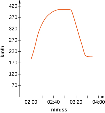
23) [T] Use the graph to estimate the velocity every 20 sec and fit to a graph of the form $v(t)=ae^{bx}\sin(cx)+d.$ (Hint: Consider the time units.)

24) [T] Using your function from the previous problem, find exactly how far the Bugati Veyron traveled in the 1 min 40 sec included in the graph.

Answer

Answers may vary. Ex: $9.405$ km