10.E: Power Series (Exercises)

10.1: Power Series and Functions

In the following exercises, state whether each statement is true, or give an example to show that it is false.

1) If \(\displaystyle \sum_{n=1}^∞a_nx^n\) converges, then \(\displaystyle a_nx^n→0\) as \(\displaystyle n→∞.\)

Solution:True. If a series converges then its terms tend to zero.

2) \(\displaystyle \sum_{n=1}^∞a_nx^n\) converges at \(\displaystyle x=0\) for any real numbers \(\displaystyle a_n\).

3) Given any sequence \(\displaystyle a_n\), there is always some \(\displaystyle R>0\), possibly very small, such that \(\displaystyle \sum_{n=1}^∞a_nx^n\) converges on \(\displaystyle (−R,R)\).

Solution: False. It would imply that \(\displaystyle a_nx^n→0\) for \(\displaystyle |x|<R\). If \(\displaystyle a_n=n^n\), then \(\displaystyle a_nx^n=(nx)^n\) does not tend to zero for any \(\displaystyle x≠0\).

4) If \(\displaystyle \sum_{n=1}^∞a_nx^n\) has radius of convergence \(\displaystyle R>0\) and if \(\displaystyle |b_n|≤|a_n|\) for all \(\displaystyle n\), then the radius of convergence of \(\displaystyle \sum_{n=1}^∞b_nx^n\) is greater than or equal to \(\displaystyle R\).

5) Suppose that \(\displaystyle \sum_{n=0}^∞a_n(x−3)^n\) converges at \(\displaystyle x=6\). At which of the following points must the series also converge? Use the fact that if \(\displaystyle \sum a_n(x−c)^n\) converges at \(\displaystyle x\), then it converges at any point closer to \(\displaystyle c\) than \(\displaystyle x\).

a. \(\displaystyle x=1\)

b. \(\displaystyle x=2\)

c. \(\displaystyle x=3\)

d. \(\displaystyle x=0\)

e. \(\displaystyle x=5.99\)

f. \(\displaystyle x=0.000001\)

Solution: It must converge on \(\displaystyle (0,6]\) and hence at: a. \(\displaystyle x=1\); b. \(\displaystyle x=2\); c. \(\displaystyle x=3\); d. \(\displaystyle x=0\); e. \(\displaystyle x=5.99\); and f. \(\displaystyle x=0.000001\).

6) Suppose that \(\displaystyle \sum_{n=0}^∞a_n(x+1)^n\) converges at \(\displaystyle x=−2\). At which of the following points must the series also converge? Use the fact that if \(\displaystyle \sum a_n(x−c)^n\) converges at \(\displaystyle x\), then it converges at any point closer to \(\displaystyle c\) than \(\displaystyle x\).

a. \(\displaystyle x=2\)

b. \(\displaystyle x=−1\)

c. \(\displaystyle x=−3\)

d. \(\displaystyle x=0\)

e. \(\displaystyle x=0.99\)

f. \(\displaystyle x=0.000001\)

In the following exercises, suppose that \(\displaystyle ∣\frac{a_{n+1}}{a_n}∣→1\) as \(\displaystyle n→∞.\) Find the radius of convergence for each series.

7) \(\displaystyle \sum_{n=0}^∞a_n2^nx^n\)

Solution: \(\displaystyle ∣\frac{a_{n+1}2^{n+1}x^{n+1}}{a_n2^nx^n}∣ =2|x|∣\frac{a_{n+1}}{a_n}∣→2|x|\) so \(\displaystyle R=\frac{1}{2}\)

8) \(\displaystyle \sum_{n=0}^∞\frac{a_nx^n}{2^n}\)

9) \(\displaystyle \sum_{n=0}^∞\frac{a_nπ^nx^n}{e^n}\)

Solution: \(\displaystyle ∣\frac{a_{n+1}(\frac{π}{e})^{n+1}x^{n+1}}{a_n(\frac{π}{e})^nx^n}∣ =\frac{π|x|}{e}∣\frac{a_{n+1}}{a_n}∣→\frac{π|x|}{e}\) so \(\displaystyle R=\frac{e}{π}\)

10) \(\displaystyle sum_{n=0}^∞\frac{a_n(−1)^nx^n}{10^n}\)

11) \(\displaystyle \sum_{n=0}^∞a_n(−1)^nx^{2n}\)

Solution: \(\displaystyle ∣\frac{a_{n+1}(−1)^{n+1}x^{2n+2}}{a_n(−1)^nx^{2n}}∣ =∣x^2∣∣\frac{a_{n+1}}{a_n}∣→∣x^2∣\) so \(\displaystyle R=1\)

12) \(\displaystyle \sum_{n=0}^∞a_n(−4)^nx^{2n}\)

In the following exercises, find the radius of convergence \(\displaystyle R\) and interval of convergence for \(\displaystyle \sum a_nx^n\) with the given coefficients \(\displaystyle a_n\).

13) \(\displaystyle \sum_{n=1}^∞\frac{(2x)^n}{n}\)

Solution: \(\displaystyle a_n=\frac{2^n}{n}\) so \(\displaystyle \frac{a_{n+1}x}{a_n}→2x\). so \(\displaystyle R=\frac{1}{2}\). When \(\displaystyle x=\frac{1}{2}\) the series is harmonic and diverges. When \(\displaystyle x=−\frac{1}{2}\) the series is alternating harmonic and converges. The interval of convergence is \(\displaystyle I=[−\frac{1}{2},\frac{1}{2})\).

14) \(\displaystyle \sum_{n=1}^∞(−1)^n\frac{x^n}{\sqrt{n}}\)

15) \(\displaystyle \sum_{n=1}^∞\frac{nx^n}{2^n}\)

Solution: \(\displaystyle a_n=\frac{n}{2^n}\) so \(\displaystyle \frac{a_{n+1}x}{a_n}→\frac{x}{2}\) so \(\displaystyle R=2\). When \(\displaystyle x=±2\) the series diverges by the divergence test. The interval of convergence is \(\displaystyle I=(−2,2)\).

16) \(\displaystyle \sum_{n=1}^∞\frac{nx^n}{e^n}\)

17) \(\displaystyle \sum_{n=1}^∞\frac{n^2x^n}{2^n}\)

Soluton: \(\displaystyle a_n=\frac{n^2}{2^n}\) so \(\displaystyle R=2\). When \(\displaystyle x=±2\) the series diverges by the divergence test. The interval of convergence is \(\displaystyle I=(−2,2).\)

18) \(\displaystyle \sum_{k=1}^∞\frac{k^ex^k}{e^k}\)

19) \(\displaystyle \sum_{k=1}^∞\frac{π^kx^k}{k^π}\)

Solution: \(\displaystyle a_k=\frac{π^k}{k^π}\) so \(\displaystyle R=\frac{1}{π}\). When \(\displaystyle x=±\frac{1}{π}\) the series is an absolutely convergent p-series. The interval of convergence is \(\displaystyle I=[−\frac{1}{π},\frac{1}{π}].\)

20) \(\displaystyle \sum_{n=1}^∞\frac{x^n}{n!}\)

21) \(\displaystyle \sum_{n=1}^∞\frac{10^nx^n}{n!}\)

Solution: \(\displaystyle a_n=\frac{10^n}{n!},\frac{a_{n+1}x}{a_n}=\frac{10x}{n+1}→0<1\) so the series converges for all \(\displaystyle x\) by the ratio test and \(\displaystyle I=(−∞,∞)\).

22) \(\displaystyle \sum_{n=1}^∞(−1)^n\frac{x^n}{ln(2n)}\)

In the following exercises, find the radius of convergence of each series.

23) \(\displaystyle \sum_{k=1}^∞\frac{(k!)^2x^k}{(2k)!}\)

Solution: \(\displaystyle a_k=\frac{(k!)^2}{(2k)!}\) so \(\displaystyle \frac{a_{k+1}}{a_k}=\frac{(k+1)^2}{(2k+2)(2k+1)}→\frac{1}{4}\) so \(\displaystyle R=4\)

24) \(\displaystyle \sum_{n=1}^∞\frac{(2n)!x^n}{n^{2n}}\)

25) \(\displaystyle \sum_{k=1}^∞\frac{k!}{1⋅3⋅5⋯(2k−1)}x^k\)

Solution: \(\displaystyle a_k=\frac{k!}{1⋅3⋅5⋯(2k−1)}\) so \(\displaystyle \frac{a_{k+1}}{a_k}=\frac{k+1}{2k+1}→\frac{1}{2}\) so \(\displaystyle R=2\)

26) \(\displaystyle \sum_{k=1}^∞\frac{2⋅4⋅6⋯2k}{(2k)!}x^k\)

27) \(\displaystyle \sum_{n=1}^∞\frac{x^n}{(^{2n}_n)}\) where \(\displaystyle (^n_k)=\frac{n!}{k!(n−k)!}\)

Solution: \(\displaystyle a_n=\frac{1}{(^{2n}_n)}\) so \(\displaystyle \frac{a_{n+1}}{a_n}=\frac{((n+1)!)^2}{(2n+2)!}\frac{2n!}{(n!)^2}=\frac{(n+1)^2}{(2n+2)(2n+1)}→\frac{1}{4}\) so \(\displaystyle R=4\)

28) \(\displaystyle \sum_{n=1}^∞sin^2nx^n\)

In the following exercises, use the ratio test to determine the radius of convergence of each series.

29) \(\displaystyle \sum_{n=1}^∞\frac{(n!)^3}{(3n)!}x^n\)

Solution: \(\displaystyle \frac{a_{n+1}}{a_n}=\frac{(n+1)^3}{(3n+3)(3n+2)(3n+1)}→\frac{1}{27}\) so \(\displaystyle R=27\)

30) \(\displaystyle \sum_{n=1}^∞\frac{2^{3n}(n!)^3}{(3n)!}x^n\)

31) \(\displaystyle \sum_{n=1}^∞\frac{n!}{n^n}x^n\)

Solution: \(\displaystyle a_n=\frac{n!}{n^n}\) so \(\displaystyle \frac{a_{n+1}}{a_n}=\frac{(n+1)!}{n!}\frac{n^n}{(n+1)^{n+1}}=(\frac{n}{n+1})^n→\frac{1}{e}\) so \(\displaystyle R=e\)

32) \(\displaystyle \sum_{n=1}^∞\frac{(2n)!}{n^{2n}}x^n\)

In the following exercises, given that \(\displaystyle \frac{1}{1−x}=\sum_{n=0}^∞x^n\) with convergence in \(\displaystyle (−1,1)\), find the power series for each function with the given center a, and identify its interval of convergence.

33) \(\displaystyle f(x)=\frac{1}{x};a=1\) (Hint: \(\displaystyle \frac{1}{x}=\frac{1}{1−(1−x)})\)

Solution: \(\displaystyle f(x)=\sum_{n=0}^∞(1−x)^n\) on \(\displaystyle I=(0,2)\)

34) \(\displaystyle f(x)=\frac{1}{1−x^2};a=0\)

35) \(\displaystyle f(x)=\frac{x}{1−x^2};a=0\)

Solution: \(\displaystyle \sum_{n=0}^∞x^{2n+1}\) on \(\displaystyle I=(−1,1)\)

36) \(\displaystyle f(x)=\frac{1}{1+x^2};a=0\)

37) \(\displaystyle f(x)=\frac{x^2}{1+x^2};a=0\)

Solution: \(\displaystyle \sum_{n=0}^∞(−1)^nx^{2n+2}\) on \(\displaystyle I=(−1,1)\)

38) \(\displaystyle f(x)=\frac{1}{2−x};a=1\)

39) \(\displaystyle f(x)=\frac{1}{1−2x};a=0.\)

Solution: \(\displaystyle \sum_{n=0}^∞2^nx^n\) on \(\displaystyle (−\frac{1}{2},\frac{1}{2})\)

40) \(\displaystyle f(x)=\frac{1}{1−4x^2};a=0\)

41) \(\displaystyle f(x)=\frac{x^2}{1−4x^2};a=0\)

Solution: \(\displaystyle \sum_{n=0}^∞4^nx^{2n+2}\) on \(\displaystyle (−\frac{1}{2},\frac{1}{2})\)

42) \(\displaystyle f(x)=\frac{x^2}{5−4x+x^2};a=2\)

Use the next exercise to find the radius of convergence of the given series in the subsequent exercises.

43) Explain why, if \(\displaystyle |a_n|^{1/n}→r>0,\) then \(\displaystyle |a_nx^n|^{1/n}→|x|r<1\) whenever \(\displaystyle |x|<\frac{1}{r}\) and, therefore, the radius of convergence of \(\displaystyle \sum_{n=1}^∞a_nx^n\) is \(\displaystyle R=\frac{1}{r}\).

Solution: \(\displaystyle |a_nx^n|^{1/n}=|a_n|^{1/n}|x|→|x|r\) as \(\displaystyle n→∞\) and \(\displaystyle |x|r<1\) when \(\displaystyle |x|<\frac{1}{r}\). Therefore, \(\displaystyle \sum_{n=1}^∞a_nx^n\) converges when \(\displaystyle |x|<\frac{1}{r}\) by the nth root test.

44) \(\displaystyle \sum_{n=1}^∞\frac{x^n}{n^n}\)

45) \(\displaystyle \sum_{k=1}^∞(\frac{k−1}{2k+3})^kx^k\)

Solution: \(\displaystyle a_k=(\frac{k−1}{2k+3})^k\) so \(\displaystyle (a_k)^{1/k}→\frac{1}{2}<1\) so \(\displaystyle R=2\)

46) \(\displaystyle \sum_{k=1}^∞(\frac{2k^2−1}{k^2+3})^kx^k\)

47) \(\displaystyle \sum_{n=1}^∞a_n=(n^{1/n}−1)^nx^n\)

Solution: \(\displaystyle a_n=(n^{1/n}−1)^n\) so \(\displaystyle (a_n)^{1/n}→0\) so \(\displaystyle R=∞\)

48) Suppose that \(\displaystyle p(x)=\sum_{n=0}^∞a_nx^n\) such that \(\displaystyle a_n=0\) if \(\displaystyle n\) is even. Explain why \(\displaystyle p(x)=p(−x).\)

49) Suppose that \(\displaystyle p(x)=\sum_{n=0}^∞a_nx^n\) such that \(\displaystyle a_n=0\) if \(\displaystyle n\) is odd. Explain why \(\displaystyle p(x)=−p(−x).\)

Solution: We can rewrite \(\displaystyle p(x)=\sum_{n=0}^∞a_{2n+1}x^{2n+1}\) and \(\displaystyle p(x)=p(−x)\) since \(\displaystyle x^{2n+1}=−(−x)^{2n+1}\).

50) Suppose that \(\displaystyle p(x)=\sum_{n=0}^∞a_nx^n\) converges on \(\displaystyle (−1,1]\). Find the interval of convergence of \(\displaystyle p(Ax)\).

51) Suppose that \(\displaystyle p(x)=\sum_{n=0}^∞a_nx^n\) converges on \(\displaystyle (−1,1]\). Find the interval of convergence of \(\displaystyle p(2x−1)\).

Solution: If \(\displaystyle x∈[0,1],\) then \(\displaystyle y=2x−1∈[−1,1]\) so \(\displaystyle p(2x−1)=p(y)=\sum_{n=0}^∞a_ny^n\) converges.

In the following exercises, suppose that \(\displaystyle p(x)=\sum_{n=0}^∞a_nx^n\) satisfies \(\displaystyle \lim_{n→∞}\frac{a_{n+1}}{a_n}=1\) where \(\displaystyle a_n≥0\) for each \(\displaystyle n\). State whether each series converges on the full interval \(\displaystyle (−1,1)\), or if there is not enough information to draw a conclusion. Use the comparison test when appropriate.

52) \(\displaystyle \sum_{n=0}^∞a_nx^{2n}\)

53) \(\displaystyle \sum_{n=0}^∞a_{2n}x^{2n}\)

Solution: Converges on \(\displaystyle (−1,1)\) by the ratio test

54) \(\displaystyle \sum_{n=0}^∞a_{2n}x^n\) (Hint:\(\displaystyle x=±\sqrt{x^2}\))

55) \(\displaystyle \sum_{n=0}^∞a_{n^2}x^{n^2}\) (Hint: Let \(\displaystyle b_k=a_k\) if \(\displaystyle k=n^2\) for some \(\displaystyle n\), otherwise \(\displaystyle b_k=0\).)

Solution: Consider the series \(\displaystyle \sum b_kx^k\) where \(\displaystyle b_k=a_k\) if \(\displaystyle k=n^2\) and \(\displaystyle b_k=0\) otherwise. Then \(\displaystyle b_k≤a_k\) and so the series converges on \(\displaystyle (−1,1)\) by the comparison test.

56) Suppose that \(\displaystyle p(x)\) is a polynomial of degree \(\displaystyle N\). Find the radius and interval of convergence of \(\displaystyle \sum_{n=1}^∞p(n)x^n\).

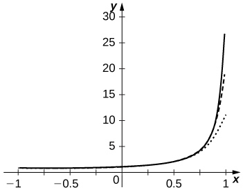
57) [T] Plot the graphs of \(\displaystyle \frac{1}{1−x}\) and of the partial sums \(\displaystyle S_N=\sum_{n=0}^Nx^n\) for \(\displaystyle n=10,20,30\) on the interval \(\displaystyle [−0.99,0.99]\). Comment on the approximation of \(\displaystyle \frac{1}{1−x}\) by \(\displaystyle S_N\) near \(\displaystyle x=−1\) and near \(\displaystyle x=1\) as \(\displaystyle N\) increases.

Solution: The approximation is more accurate near \(\displaystyle x=−1\). The partial sums follow \(\displaystyle \frac{1}{1−x}\) more closely as \(\displaystyle N\) increases but are never accurate near \(\displaystyle x=1\) since the series diverges there.

58) [T] Plot the graphs of \(\displaystyle −ln(1−x)\) and of the partial sums \(\displaystyle S_N=\sum_{n=1}^N\frac{x^n}{n}\) for \(\displaystyle n=10,50,100\) on the interval \(\displaystyle [−0.99,0.99]\). Comment on the behavior of the sums near \(\displaystyle x=−1\) and near \(\displaystyle x=1\) as \(\displaystyle N\) increases.

59) [T] Plot the graphs of the partial sums \(\displaystyle S_n=\sum_{n=1}^N\frac{x^n}{n^2}\) for \(\displaystyle n=10,50,100\) on the interval \(\displaystyle [−0.99,0.99]\). Comment on the behavior of the sums near \(\displaystyle x=−1\) and near \(\displaystyle x=1\) as \(\displaystyle N\) increases.

Solution: The approximation appears to stabilize quickly near both \(\displaystyle x=±1\).

60) [T] Plot the graphs of the partial sums \(\displaystyle S_N=\sum_{n=1}^Nsinnx^n\) for \(\displaystyle n=10,50,100\) on the interval \(\displaystyle [−0.99,0.99]\). Comment on the behavior of the sums near \(\displaystyle x=−1\) and near \(\displaystyle x=1\) as \(\displaystyle N\) increases.

61) [T] Plot the graphs of the partial sums \(\displaystyle S_N=\sum_{n=0}^N(−1)^n\frac{x^{2n+1}}{(2n+1)!}\) for \(\displaystyle n=3,5,10\) on the interval \(\displaystyle [−2π,2π]\). Comment on how these plots approximate \(\displaystyle sinx\) as \(\displaystyle N\) increases.

Solution: The polynomial curves have roots close to those of \(\displaystyle sinx\) up to their degree and then the polynomials diverge from \(\displaystyle sinx\).

62) [T] Plot the graphs of the partial sums \(\displaystyle S_N=\sum_{n=0}^N(−1)^n\frac{x^{2n}}{(2n)!}\) for \(\displaystyle n=3,5,10\) on the interval \(\displaystyle [−2π,2π]\). Comment on how these plots approximate \(\displaystyle cosx\) as \(\displaystyle N\) increases.

10.2: Properties of Power Series

1) If \(\displaystyle f(x)=\sum_{n=0}^∞\frac{x^n}{n!}\) and \(\displaystyle g(x)=\sum_{n=0}^∞(−1)^n\frac{x^n}{n!}\), find the power series of \(\displaystyle \frac{1}{2}(f(x)+g(x))\) and of \(\displaystyle \frac{1}{2}(f(x)−g(x))\).

Solution: \(\displaystyle \frac{1}{2}(f(x)+g(x))=\sum_{n=0}^∞\frac{x^{2n}}{(2n)!}\) and \(\displaystyle \frac{1}{2}(f(x)−g(x))=\sum_{n=0}^∞\frac{x^{2n+1}}{(2n+1)!}\).

2) If \(\displaystyle C(x)=\sum_{n=0}^∞\frac{x^{2n}}{(2n)!}\) and \(\displaystyle S(x)=\sum_{n=0}^∞\frac{x^{2n+1}}{(2n+1)!}\), find the power series of \(\displaystyle C(x)+S(x)\) and of \(\displaystyle C(x)−S(x)\).

In the following exercises, use partial fractions to find the power series of each function.

3) \(\displaystyle \frac{4}{(x−3)(x+1)}\)

Solution: \(\displaystyle \frac{4}{(x−3)(x+1)}=\frac{1}{x−3}−\frac{1}{x+1}=−\frac{1}{3(1−\frac{x}{3})}−\frac{1}{1−(−x)}=−\frac{1}{3}\sum_{n=0}^∞(\frac{x}{3})^n−\sum_{n=0}^∞(−1)^nx^n=\sum_{n=0}^∞((−1)^{n+1}−\frac{1}{3n+1})x^n\)

4) \(\displaystyle \frac{3}{(x+2)(x−1)}\)

5) \(\displaystyle \frac{5}{(x^2+4)(x^2−1)}\)

Soution: \(\displaystyle \frac{5}{(x^2+4)(x^2−1)}=\frac{1}{x^2−1}−\frac{1}{4}\frac{1}{1+(\frac{x}{2})^2}=−\sum_{n=0}^∞x^{2n}−\frac{1}{4}\sum_{n=0}^∞(−1)^n(\frac{x}{2})^n=\sum_{n=0}^∞((−1)+(−1)^{n+1}\frac{1}{2^{n+2}})x^{2n}\)

6) \(\displaystyle \frac{30}{(x^2+1)(x^2−9)}\)

In the following exercises, express each series as a rational function.

7) \(\displaystyle \sum_{n=1}^∞\frac{1}{x^n}\)

Solution: \(\displaystyle \frac{1}{x}\sum_{n=0}^∞\frac{1}{x^n}=\frac{1}{x}\frac{1}{1−\frac{1}{x}}=\frac{1}{x−1}\)

8) \(\displaystyle \sum_{n=1}^∞\frac{1}{x^{2n}}\)

9) \(\displaystyle \sum_{n=1}^∞\frac{1}{(x−3)^{2n−1}}\)

Solution: \(\displaystyle \frac{1}{x−3}\frac{1}{1−\frac{1}{(x−3)^2}}=\frac{x−3}{(x−3)^2−1}\)

10) \(\displaystyle \sum_{n=1}^∞(\frac{1}{(x−3)^{2n−1}}−\frac{1}{(x−2)^{2n−1}})\)

The following exercises explore applications of annuities.

11) Calculate the present values P of an annuity in which $10,000 is to be paid out annually for a period of 20 years, assuming interest rates of \(\displaystyle r=0.03,r=0.05\), and \(\displaystyle r=0.07\).

Solution: \(\displaystyle P=P_1+⋯+P_{20}\) where \(\displaystyle P_k=10,000\frac{1}{(1+r)^k}\). Then \(\displaystyle P=10,000\sum_{k=1}^{20}\frac{1}{(1+r)^k}=10,000\frac{1−(1+r)^{−20}}{r}\). When \(\displaystyle r=0.03,P≈10,000×14.8775=148,775.\) When \(\displaystyle r=0.05,P≈10,000×12.4622=124,622.\) When \(\displaystyle r=0.07,P≈105,940\).

12) Calculate the present values P of annuities in which $9,000 is to be paid out annually perpetually, assuming interest rates of \(\displaystyle r=0.03,r=0.05\) and \(\displaystyle r=0.07\).

13) Calculate the annual payouts C to be given for 20 years on annuities having present value $100,000 assuming respective interest rates of \(\displaystyle r=0.03,r=0.05,\) and \(\displaystyle r=0.07.\)

Solution: In general, \(\displaystyle P=\frac{C(1−(1+r)^{−N})}{r}\) for N years of payouts, or \(\displaystyle C=\frac{Pr}{1−(1+r)^{−N}}\). For \(\displaystyle N=20\) and \(\displaystyle P=100,000\), one has \(\displaystyle C=6721.57\) when \(\displaystyle r=0.03;C=8024.26\) when \(\displaystyle r=0.05\); and \(\displaystyle C≈9439.29\) when \(\displaystyle r=0.07\).

14) Calculate the annual payouts C to be given perpetually on annuities having present value $100,000 assuming respective interest rates of \(\displaystyle r=0.03,r=0.05,\) and \(\displaystyle r=0.07\).

15) Suppose that an annuity has a present value \(\displaystyle P=1\) million dollars. What interest rate r would allow for perpetual annual payouts of $50,000?

Solution: In general, \(\displaystyle P=\frac{C}{r}.\) Thus, \(\displaystyle r=\frac{C}{P}=5×\frac{10^4}{10^6}=0.05.\)

16) Suppose that an annuity has a present value \(\displaystyle P=10\) million dollars. What interest rate r would allow for perpetual annual payouts of $100,000?

In the following exercises, express the sum of each power series in terms of geometric series, and then express the sum as a rational function.

17) \(\displaystyle x+x^2−x^3+x^4+x^5−x^6+⋯\) (Hint: Group powers \(\displaystyle x^{3k}, x^{3k−1},\) and \(\displaystyle x^{3k−2}\).)

Solution: \(\displaystyle (x+x^2−x^3)(1+x^3+x^6+⋯)=\frac{x+x^2−x^3}{1−x^3}\)

18) \(\displaystyle x+x^2−x^3−x^4+x^5+x^6−x^7−x^8+⋯\) (Hint: Group powers \(\displaystyle x^{4k}, x^{4k−1},\) etc.)

19) \(\displaystyle x−x^2−x^3+x^4−x^5−x^6+x^7−⋯\) (Hint: Group powers \(\displaystyle x^{3k}, x^{3k−1}\), and \(\displaystyle x^{3k−2}\).)

Solution: \(\displaystyle (x−x^2−x^3)(1+x^3+x^6+⋯)=\frac{x−x^2−x^3}{1−x^3}\)

20) \(\displaystyle \frac{x}{2}+\frac{x^2}{4}−\frac{x^3}{8}+\frac{x^4}{16}+\frac{x^5}{32}−\frac{x^6}{64}+⋯\) (Hint: Group powers \(\displaystyle \frac{x}{2})^{3k},(\frac{x}{2})^{3k−1},\) and \(\displaystyle \frac{x}{2})^{3k−2}\).)

In the following exercises, find the power series of \(\displaystyle f(x)g(x)\) given f and g as defined.

21) \(\displaystyle f(x)=2\sum_{n=0}^∞x^n,g(x)=\sum_{n=0}^∞nx^n\)

Solution: \(\displaystyle a_n=2,b_n=n\) so \(\displaystyle c_n=\sum_{k=0}^nb_ka_{n−k}=2\sum_{k=0}^nk=(n)(n+1)\) and \(\displaystyle f(x)g(x)=\sum_{n=1}^∞n(n+1)x^n\)

22) \(\displaystyle f(x)=\sum_{n=1}^∞x^n,g(x)=\sum_{n=1}^∞\frac{1}{n}x^n\). Express the coefficients of \(\displaystyle f(x)g(x)\) in terms of \(\displaystyle H_n=\sum_{k=1}^n\frac{1}{k}\).

23) \(\displaystyle f(x)=g(x)=\sum_{n=1}^∞(\frac{x}{2})^n\)

Solution: \(\displaystyle a_n=b_n=2^{−n}\) so \(\displaystyle c_n=\sum_{k=1}^nb_ka_{n−k}=2^{−n}\sum_{k=1}^n1=\frac{n}{2^n}\) and \(\displaystyle f(x)g(x)=\sum_{n=1}^∞n(\frac{x}{2})^n\)

24) \(\displaystyle f(x)=g(x)=\sum_{n=1}^∞nx^n\)

In the following exercises, differentiate the given series expansion of f term-by-term to obtain the corresponding series expansion for the derivative of f.

25) \(\displaystyle f(x)=\frac{1}{1+x}=\sum_{n=0}^∞(−1)^nx^n\)

Solution: The derivative of \(\displaystyle f\) is \(\displaystyle −\frac{1}{(1+x)^2}=−\sum_{n=0}^∞(−1)^n(n+1)x^n\).

26) \(\displaystyle f(x)=\frac{1}{1−x^2}=\sum_{n=0}^∞x^{2n}\)

In the following exercises, integrate the given series expansion of \(\displaystyle f\) term-by-term from zero to x to obtain the corresponding series expansion for the indefinite integral of \(\displaystyle f\).

27) \(\displaystyle f(x)=\frac{2x}{(1+x^2)^2}=\sum_{n=1}^∞(−1)^n(2n)x^{2n−1}\)

Solution: The indefinite integral of \(\displaystyle f\) is \(\displaystyle \frac{1}{1+x^2}=\sum_{n=0}^∞(−1)^nx^{2n}\).

28) \(\displaystyle f(x)=\frac{2x}{1+x^2}=2\sum_{n=0}^∞(−1)^nx^{2n+1}\)

In the following exercises, evaluate each infinite series by identifying it as the value of a derivative or integral of geometric series.

29) Evaluate \(\displaystyle \sum_{n=1}^∞\frac{n}{2^n}\) as \(\displaystyle f′(\frac{1}{2})\) where \(\displaystyle f(x)=\sum_{n=0}^∞x^n\).

Solution: \(\displaystyle f(x)=\sum_{n=0}^∞x^n=\frac{1}{1−x};f′(\frac{1}{2})=\sum_{n=1}^∞\frac{n}{2^{n−1}}=\frac{d}{dx}(1−x)^{−1}∣_{x=1/2}=\frac{1}{(1−x)^2}∣_{x=1/2}=4\) so \(\displaystyle \sum_{n=1}^∞\frac{n}{2^n}=2.\)

30) Evaluate \(\displaystyle \sum_{n=1}^∞\frac{n}{3^n}\) as \(\displaystyle f′(\frac{1}{3})\) where \(\displaystyle f(x)=\sum_{n=0}^∞x6n\).

31) Evaluate \(\displaystyle \sum_{n=2}^∞\frac{n(n−1)}{2^n}\) as \(\displaystyle f''(\frac{1}{2})\) where \(\displaystyle f(x)=\sum_{n=0}^∞x^n\).

Solution: \(\displaystyle f(x)=\sum_{n=0}^∞x^n=\frac{1}{1−x};f''(\frac{1}{2})=\sum_{n=2}^∞\frac{n(n−1)}{2^{n−2}}=\frac{d^2}{dx^2}(1−x)^{−1}∣_{x=1/2}=\frac{2}{(1−x)^3}∣_{x=1/2}=16\) so \(\displaystyle \sum_{n=2}^∞n\frac{(n−1)}{2^n}=4.\)

32) Evaluate \(\displaystyle \sum_{n=0}^∞\frac{(−1)^n}{n+1}\) as \(\displaystyle ∫^1_0f(t)dt\) where \(\displaystyle f(x)=\sum_{n=0}^∞(−1)^nx^{2n}=\frac{1}{1+x^2}\).

In the following exercises, given that \(\displaystyle \frac{1}{1−x}=\sum_{n=0}^∞x^n\), use term-by-term differentiation or integration to find power series for each function centered at the given point.

33) \(\displaystyle f(x)=lnx\) centered at \(\displaystyle x=1\) (Hint: \(\displaystyle x=1−(1−x)\))

Solution: \(\displaystyle ∫\sum(1−x)^ndx=∫\sum(−1)^n(x−1)^ndx=\sum \frac{(−1)^n(x−1)^{n+1}}{n+1}\)

34) \(\displaystyle ln(1−x)\) at \(\displaystyle x=0\)

35) \(\displaystyle ln(1−x^2)\) at \(\displaystyle x=0\)

Solution: \(\displaystyle −∫^{x^2}_{t=0}\frac{1}{1−t}dt=−\sum_{n=0}^∞∫^{x^2}_0t^ndx−\sum_{n=0}^∞\frac{x^{2(n+1)}}{n+1}=−\sum_{n=1}^∞\frac{x^{2n}}{n}\)

36) \(\displaystyle f(x)=\frac{2x}{(1−x^2)^2}\) at \(\displaystyle x=0\)

37) \(\displaystyle f(x)=tan^{−1}(x^2)\) at \(\displaystyle x=0\)

Solution: \(\displaystyle ∫^{x^2}_0\frac{dt}{1+t^2}=\sum_{n=0}^∞(−1)^n∫^{x^2}_0t^{2n}dt=\sum_{n=0}^∞(−1)^n\frac{t^{2n+1}}{2n+1}∣^{x^2}_{t=0}=\sum_{n=0}^∞(−1)^n\frac{x^{4n+2}}{2n+1}\)

38) \(\displaystyle f(x)=ln(1+x^2)\) at \(\displaystyle x=0\)

39) \(\displaystyle f(x)=∫^x_0lntdt\) where \(\displaystyle ln(x)=\sum_{n=1}^∞(−1)^{n−1}\frac{(x−1)^n}{n}\)

Solution: Term-by-term integration gives \(\displaystyle ∫^x_0lntdt=\sum_{n=1}^∞(−1)^{n−1}\frac{(x−1)^{n+1}}{n(n+1)}=\sum_{n=1}^∞(−1)^{n−1}(\frac{1}{n}−\frac{1}{n+1})(x−1)^{n+1}=(x−1)lnx+\sum_{n=2}^∞(−1)^n\frac{(x−1)^n}{n}=xlnx−x.\)

40) [T] Evaluate the power series expansion \(\displaystyle ln(1+x)=\sum_{n=1}^∞(−1)^{n−1}\frac{x^n}{n}\) at \(\displaystyle x=1\) to show that \(\displaystyle ln(2)\) is the sum of the alternating harmonic series. Use the alternating series test to determine how many terms of the sum are needed to estimate \(\displaystyle ln(2)\)

accurate to within 0.001, and find such an approximation.

41) [T] Subtract the infinite series of \(\displaystyle ln(1−x)\) from \(\displaystyle ln(1+x)\) to get a power series for \(\displaystyle ln(\frac{1+x}{1−x})\). Evaluate at \(\displaystyle x=\frac{1}{3}\). What is the smallest N such that the Nth partial sum of this series approximates \(\displaystyle ln(2)\) with an error less than 0.001?

Solution: We have \(\displaystyle ln(1−x)=−\sum_{n=1}^∞\frac{x^n}{n}\) so \(\displaystyle ln(1+x)=\sum_{n=1}^∞(−1)^{n−1}\frac{x^n}{n}\). Thus, \(\displaystyle ln(\frac{1+x}{1−x})=\sum_{n=1}^∞(1+(−1)^{n−1})\frac{x^n}{n}=2\sum_{n=1}^∞\frac{x^{2n−1}}{2n−1}\). When \(\displaystyle x=\frac{1}{3}\) we obtain \(\displaystyle ln(2)=2\sum_{n=1}^∞\frac{1}{3^{2n−1}(2n−1)}\). We have \(\displaystyle 2\sum_{n=1}^3\frac{1}{3^{2n−1}(2n−1)}=0.69300…\), while \(\displaystyle 2\sum_{n=1}^4\frac{1}{3^{2n−1}(2n−1)}=0.69313…\) and \(\displaystyle ln(2)=0.69314…;\) therefore, \(\displaystyle N=4\).

In the following exercises, using a substitution if indicated, express each series in terms of elementary functions and find the radius of convergence of the sum.

42) \(\displaystyle \sum_{k=0}^∞(x^k−x^{2k+1})\)

43) \(\displaystyle \sum_{k=1}^∞\frac{x^{3k}}{6k}\)

Solution: \(\displaystyle \sum_{k=1}^∞\frac{x^k}{k}=−ln(1−x)\) so \(\displaystyle \sum_{k=1}6∞\frac{x^{3k}}{6k}=−\frac{1}{6}ln(1−x^3)\). The radius of convergence is equal to 1 by the ratio test.

44) \(\displaystyle \sum_{k=1}^∞(1+x^2)^{−k}\) using \(\displaystyle y=\frac{1}{1+x^2}\)

45) \(\displaystyle \sum_{k=1}^∞2^{−kx}\) using \(\displaystyle y=2^{−x}\)

Solution: If \(\displaystyle y=2^{−x}\), then \(\displaystyle \sum_{k=1}^∞y^k=\frac{y}{1−y}=\frac{2^{−x}}{1−2^{−x}}=\frac{1}{2^x−1}\). If \(\displaystyle a_k=2^{−kx}\), then \(\displaystyle \frac{a_{k+1}}{a_k}=2^{−x}<1\) when \(\displaystyle x>0\). So the series converges for all \(\displaystyle x>0\).

46) Show that, up to powers \(\displaystyle x^3\) and \(\displaystyle y^3\), \(\displaystyle E(x)=\sum_{n=0}^∞\frac{x^n}{n!}\) satisfies \(\displaystyle E(x+y)=E(x)E(y)\).

47) Differentiate the series \(\displaystyle E(x)=\sum_{n=0}^∞\frac{x^n}{n!}\) term-by-term to show that \(\displaystyle E(x)\) is equal to its derivative.

Solution: Answers will vary.

48) Show that if \(\displaystyle f(x)=\sum_{n=0}^∞a_nx^n\) is a sum of even powers, that is, \(\displaystyle a_n=0\) if \(\displaystyle n\) is odd, then \(\displaystyle F=∫^x_0f(t)dt\) is a sum of odd powers, while if I is a sum of odd powers, then F is a sum of even powers.

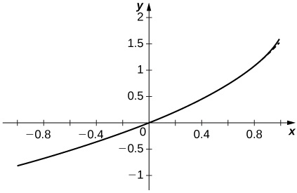
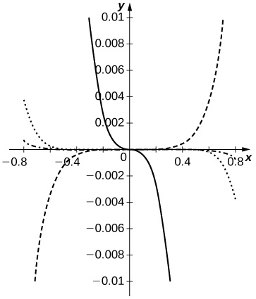
49) [T] Suppose that the coefficients an of the series \(\displaystyle \sum_{n=0}^∞a_nx^n\) are defined by the recurrence relation \(\displaystyle a_n=\frac{a_{n−1}}{n}+\frac{a_{n−2}}{n(n−1)}\). For \(\displaystyle a_0=0\) and \(\displaystyle a_1=1\), compute and plot the sums \(\displaystyle S_N=\sum_{n=0}^Na_nx^n\) for \(\displaystyle N=2,3,4,5\) on \(\displaystyle [−1,1].\)

Solution: The solid curve is \(\displaystyle S_5\). The dashed curve is \(\displaystyle S_2\), dotted is \(\displaystyle S_3\), and dash-dotted is \(\displaystyle S_4\)

50) [T] Suppose that the coefficients an of the series \(\displaystyle \sum_{n=0}^∞a_nx^n\) are defined by the recurrence relation \(\displaystyle a_n=\frac{a_{n−1}}{\sqrt{n}}−\frac{a_{n−2}}{\sqrt{n(n−1)}}\). For \(\displaystyle a_0=1\) and \(\displaystyle a_1=0\), compute and plot the sums \(\displaystyle S_N=\sum_{n=0}^Na_nx^n\) for \(\displaystyle N=2,3,4,5\) on \(\displaystyle [−1,1]\).

51) [T] Given the power series expansion \(\displaystyle ln(1+x)=\sum_{n=1}^∞(−1)^{n−1}\frac{x^n}{n}\), determine how many terms N of the sum evaluated at \(\displaystyle x=−1/2\) are needed to approximate \(\displaystyle ln(2)\) accurate to within 1/1000. Evaluate the corresponding partial sum \(\displaystyle \sum_{n=1}^N(−1)^{n−1}\frac{x^n}{n}\).

Solution: When \(\displaystyle x=−\frac{1}{2},−ln(2)=ln(\frac{1}{2})=−\sum_{n=1}^∞\frac{1}{n2^n}\). Since \(\displaystyle \sum^∞_{n=11}\frac{1}{n2^n}<\sum_{n=11}^∞\frac{1}{2^n}=\frac{1}{2^{10}},\) one has \(\displaystyle \sum_{n=1}^{10}\frac{1}{n2^n}=0.69306…\) whereas \(\displaystyle ln(2)=0.69314…;\) therefore, \(\displaystyle N=10.\)

52) [T] Given the power series expansion \(\displaystyle tan^{−1}(x)=\sum_{k=0}^∞(−1)^k\frac{x^{2k+1}}{2k+1}\), use the alternating series test to determine how many terms N of the sum evaluated at \(\displaystyle x=1\) are needed to approximate \(\displaystyle tan^{−1}(1)=\frac{π}{4}\) accurate to within 1/1000. Evaluate the corresponding partial sum \(\displaystyle \sum_{k=0}^N(−1)^k\frac{x^{2k+1}}{2k+1}\).

53) [T] Recall that \(\displaystyle tan^{−1}(\frac{1}{\sqrt{3}})=\frac{π}{6}.\) Assuming an exact value of \(\displaystyle \frac{1}{\sqrt{3}})\), estimate \(\displaystyle \frac{π}{6}\) by evaluating partial sums \(\displaystyle S_N(\frac{1}{\sqrt{3}})\) of the power series expansion \(\displaystyle tan^{−1}(x)=\sum_{k=0}^∞(−1)^k\frac{x^{2k+1}}{2k+1}\) at \(\displaystyle x=\frac{1}{\sqrt{3}}\). What is the smallest number \(\displaystyle N\) such that \(\displaystyle 6S_N(\frac{1}{\sqrt{3}})\) approximates \(\displaystyle π\) accurately to within 0.001? How many terms are needed for accuracy to within 0.00001?

Solution: \(\displaystyle 6S_N(\frac{1}{\sqrt{3}})=2\sqrt{3}\sum_{n=0}^N(−1)^n\frac{1}{3^n(2n+1).}\) One has \(\displaystyle π−6S_4(\frac{1}{\sqrt{3}})=0.00101…\) and \(\displaystyle π−6S_5(\frac{1}{\sqrt{3}})=0.00028…\) so \(\displaystyle N=5\) is the smallest partial sum with accuracy to within 0.001. Also, \(\displaystyle π−6S_7(\frac{1}{\sqrt{3}})=0.00002…\) while \(\displaystyle π−6S_8(\frac{1}{\sqrt{3}})=−0.000007…\) so \(\displaystyle N=8\) is the smallest N to give accuracy to within 0.00001.

10.3: Taylor and Maclaurin Series

Taylor Polynomials

In exercises 1 - 8, find the Taylor polynomials of degree two approximating the given function centered at the given point.

1) \( f(x)=1+x+x^2\) at \( a=1\)

2) \( f(x)=1+x+x^2\) at \( a=−1\)

Answer

\( f(−1)=1;\;f′(−1)=−1;\;f''(−1)=2;\quad p_2(x)=1−(x+1)+(x+1)^2\)

3) \( f(x)=\cos(2x)\) at \( a=π\)

4) \( f(x)=\sin(2x)\) at \( a=\frac{π}{2}\)

Answer

\( f′(x)=2\cos(2x);\;f''(x)=−4\sin(2x);\quad p_2(x)=−2(x−\frac{π}{2})\)

5) \( f(x)=\sqrt{x}\) at \( a=4\)

6) \( f(x)=\ln x\) at \( a=1\)

Answer

\( f′(x)=\dfrac{1}{x};\; f''(x)=−\dfrac{1}{x^2};\quad p_2(x)=0+(x−1)−\frac{1}{2}(x−1)^2\)

7) \( f(x)=\dfrac{1}{x}\) at \( a=1\)

8) \( f(x)=e^x\) at \( a=1\)

Answer

\( p_2(x)=e+e(x−1)+\dfrac{e}{2}(x−1)^2\)

Taylor Remainder Theorem

In exercises 9 - 14, verify that the given choice of \(n\) in the remainder estimate \( |R_n|≤\dfrac{M}{(n+1)!}(x−a)^{n+1}\), where \(M\) is the maximum value of \( ∣f^{(n+1)}(z)∣\) on the interval between \(a\) and the indicated point, yields \( |R_n|≤\frac{1}{1000}\). Find the value of the Taylor polynomial \( p_n\) of \( f\) at the indicated point.

9) [T] \( \sqrt{10};\; a=9,\; n=3\)

10) [T] \( (28)^{1/3};\; a=27,\; n=1\)

Answer

\( \dfrac{d^2}{dx^2}x^{1/3}=−\dfrac{2}{9x^{5/3}}≥−0.00092…\) when \( x≥28\) so the remainder estimate applies to the linear approximation \( x^{1/3}≈p_1(27)=3+\dfrac{x−27}{27}\), which gives \( (28)^{1/3}≈3+\frac{1}{27}=3.\bar{037}\), while \( (28)^{1/3}≈3.03658.\)

11) [T] \( \sin(6);\; a=2π,\; n=5\)

12) [T] \( e^2; \; a=0,\; n=9\)

Answer

Using the estimate \( \dfrac{2^{10}}{10!}<0.000283\) we can use the Taylor expansion of order 9 to estimate \( e^x\) at \( x=2\). as \( e^2≈p_9(2)=1+2+\frac{2^2}{2}+\frac{2^3}{6}+⋯+\frac{2^9}{9!}=7.3887\)… whereas \( e^2≈7.3891.\)

13) [T] \( \cos(\frac{π}{5});\; a=0,\; n=4\)

14) [T] \( \ln(2);\; a=1,\; n=1000\)

Answer

Since \( \dfrac{d^n}{dx^n}(\ln x)=(−1)^{n−1}\dfrac{(n−1)!}{x^n},R_{1000}≈\frac{1}{1001}\). One has \(\displaystyle p_{1000}(1)=\sum_{n=1}^{1000}\dfrac{(−1)^{n−1}}{n}≈0.6936\) whereas \( \ln(2)≈0.6931⋯.\)

Approximating Definite Integrals Using Taylor Series

15) Integrate the approximation \(\sin t≈t−\dfrac{t^3}{6}+\dfrac{t^5}{120}−\dfrac{t^7}{5040}\) evaluated at \( π\)t to approximate \(\displaystyle ∫^1_0\frac{\sin πt}{πt}\,dt\).

16) Integrate the approximation \( e^x≈1+x+\dfrac{x^2}{2}+⋯+\dfrac{x^6}{720}\) evaluated at \( −x^2\) to approximate \(\displaystyle ∫^1_0e^{−x^2}\,dx.\)

Answer

\(\displaystyle ∫^1_0\left(1−x^2+\frac{x^4}{2}−\frac{x^6}{6}+\frac{x^8}{24}−\frac{x^{10}}{120}+\frac{x^{12}}{720}\right)\,dx =1−\frac{1^3}{3}+\frac{1^5}{10}−\frac{1^7}{42}+\frac{1^9}{9⋅24}−\frac{1^{11}}{120⋅11}+\frac{1^{13}}{720⋅13}≈0.74683\) whereas \(\displaystyle ∫^1_0e^{−x^2}dx≈0.74682.\)

More Taylor Remainder Theorem Problems

In exercises 17 - 20, find the smallest value of \(n\) such that the remainder estimate \( |R_n|≤\dfrac{M}{(n+1)!}(x−a)^{n+1}\), where \(M\) is the maximum value of \( ∣f^{(n+1)}(z)∣\) on the interval between \(a\) and the indicated point, yields \( |R_n|≤\frac{1}{1000}\) on the indicated interval.

17) \( f(x)=\sin x\) on \( [−π,π],\; a=0\)

18) \( f(x)=\cos x\) on \( [−\frac{π}{2},\frac{π}{2}],\; a=0\)

Answer

Since \( f^{(n+1)}(z)\) is \(\sin z\) or \(\cos z\), we have \( M=1\). Since \( |x−0|≤\frac{π}{2}\), we seek the smallest \(n\) such that \( \dfrac{π^{n+1}}{2^{n+1}(n+1)!}≤0.001\). The smallest such value is \( n=7\). The remainder estimate is \( R_7≤0.00092.\)

19) \( f(x)=e^{−2x}\) on \( [−1,1],a=0\)

20) \( f(x)=e^{−x}\) on \( [−3,3],a=0\)

Answer

Since \( f^{(n+1)}(z)=±e^{−z}\) one has \( M=e^3\). Since \( |x−0|≤3\), one seeks the smallest \(n\) such that \( \dfrac{3^{n+1}e^3}{(n+1)!}≤0.001\). The smallest such value is \( n=14\). The remainder estimate is \( R_{14}≤0.000220.\)

In exercises 21 - 24, the maximum of the right-hand side of the remainder estimate \( |R_1|≤\dfrac{max|f''(z)|}{2}R^2\) on \( [a−R,a+R]\) occurs at \(a\) or \( a±R\). Estimate the maximum value of \(R\) such that \( \dfrac{max|f''(z)|}{2}R^2≤0.1\) on \( [a−R,a+R]\) by plotting this maximum as a function of \(R\).

21) [T] \( e^x\) approximated by \( 1+x,\; a=0\)

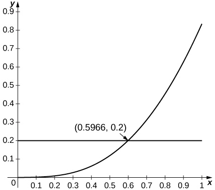
22) [T] \( \sin x\) approximated by \( x,\; a=0\)

Answer

Since \( \sin x\) is increasing for small \( x\) and since \( \frac{d^2}{dx^2}\left(\sin x\right)=−\sin x\), the estimate applies whenever \( R^2\sin(R)≤0.2\), which applies up to \( R=0.596.\)

23) [T] \( \ln x\) approximated by \( x−1,\; a=1\)

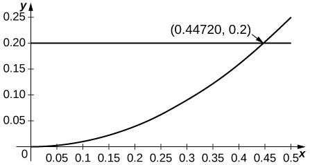
24) [T] \( \cos x\) approximated by \( 1,\; a=0\)

Answer

Since the second derivative of \( \cos x\) is \( −\cos x\) and since \( \cos x\) is decreasing away from \( x=0\), the estimate applies when \( R^2\cos R≤0.2\) or \( R≤0.447\).

Taylor Series

In exercises 25 - 35, find the Taylor series of the given function centered at the indicated point.

25) \(f(x) = x^4\) at \( a=−1\)

26) \(f(x) = 1+x+x^2+x^3\) at \( a=−1\)

Answer

\( (x+1)^3−2(x+1)^2+2(x+1)\)

27) \(f(x) = \sin x\) at \( a=π\)

28) \(f(x) = \cos x\) at \( a=2π\)

Answer

Values of derivatives are the same as for \( x=0\) so \(\displaystyle \cos x=\sum_{n=0}^∞(−1)^n\frac{(x−2π)^{2n}}{(2n)!}\)

29) \(f(x) = \sin x\) at \( x=\frac{π}{2}\)

30) \(f(x) = \cos x\) at \( x=\frac{π}{2}\)

Answer

\( \cos(\frac{π}{2})=0,\;−\sin(\frac{π}{2})=−1\) so \(\displaystyle \cos x=\sum_{n=0}^∞(−1)^{n+1}\frac{(x−\frac{π}{2})^{2n+1}}{(2n+1)!}\), which is also \( −\cos(x−\frac{π}{2})\).

31) \(f(x) = e^x\) at \( a=−1\)

32) \(f(x) = e^x\) at \( a=1\)

Answer

The derivatives are \( f^{(n)}(1)=e,\) so \(\displaystyle e^x=e\sum_{n=0}^∞\frac{(x−1)^n}{n!}.\)

33) \(f(x) = \dfrac{1}{(x−1)^2}\) at \( a=0\) (Hint: Differentiate the Taylor Series for\( \dfrac{1}{1−x}\).)

34) \(f(x) = \dfrac{1}{(x−1)^3}\) at \( a=0\)

Answer

\(\displaystyle \frac{1}{(x−1)^3}=−\frac{1}{2}\frac{d^2}{dx^2}\left(\frac{1}{1−x}\right)=−\sum_{n=0}^∞\left(\frac{(n+2)(n+1)x^n}{2}\right)\)

35) \(\displaystyle F(x)=∫^x_0\cos(\sqrt{t})\,dt;\quad \text{where}\; f(t)=\sum_{n=0}^∞(−1)^n\frac{t^n}{(2n)!}\) at a=0 (Note: \( f\) is the Taylor series of \(\cos(\sqrt{t}).)\)

In exercises 36 - 44, compute the Taylor series of each function around \( x=1\).

36) \( f(x)=2−x\)

Answer

\( 2−x=1−(x−1)\)

37) \( f(x)=x^3\)

38) \( f(x)=(x−2)^2\)

Answer

\( ((x−1)−1)^2=(x−1)^2−2(x−1)+1\)

39) \( f(x)=\ln x\)

40) \( f(x)=\dfrac{1}{x}\)

Answer

\(\displaystyle \frac{1}{1−(1−x)}=\sum_{n=0}^∞(−1)^n(x−1)^n\)

41) \( f(x)=\dfrac{1}{2x−x^2}\)

42) \( f(x)=\dfrac{x}{4x−2x^2−1}\)

Answer

\(\displaystyle x\sum_{n=0}^∞2^n(1−x)^{2n}=\sum_{n=0}^∞2^n(x−1)^{2n+1}+\sum_{n=0}^∞2^n(x−1)^{2n}\)

43) \( f(x)=e^{−x}\)

44) \( f(x)=e^{2x}\)

Answer

\(\displaystyle e^{2x}=e^{2(x−1)+2}=e^2\sum_{n=0}^∞\frac{2^n(x−1)^n}{n!}\)

Maclaurin Series

[T] In exercises 45 - 48, identify the value of \(x\) such that the given series \(\displaystyle \sum_{n=0}^∞a_n\) is the value of the Maclaurin series of \( f(x)\) at \( x\). Approximate the value of \( f(x)\) using \(\displaystyle S_{10}=\sum_{n=0}^{10}a_n\).

45) \(\displaystyle \sum_{n=0}^∞\frac{1}{n!}\)

46) \(\displaystyle \sum_{n=0}^∞\frac{2^n}{n!}\)

Answer

\( x=e^2;\quad S_{10}=\dfrac{34,913}{4725}≈7.3889947\)

47) \(\displaystyle \sum_{n=0}^∞\frac{(−1)^n(2π)^{2n}}{(2n)!}\)

48) \(\displaystyle \sum_{n=0}^∞\frac{(−1)^n(2π)^{2n+1}}{(2n+1)!}\)

Answer

\(\sin(2π)=0;\quad S_{10}=8.27×10^{−5}\)

In exercises 49 - 52 use the functions \( S_5(x)=x−\dfrac{x^3}{6}+\dfrac{x^5}{120}\) and \( C_4(x)=1−\dfrac{x^2}{2}+\dfrac{x^4}{24}\) on \( [−π,π]\).

49) [T] Plot \(\sin^2x−(S_5(x))^2\) on \( [−π,π]\). Compare the maximum difference with the square of the Taylor remainder estimate for \( \sin x.\)

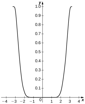
50) [T] Plot \(\cos^2x−(C_4(x))^2\) on \( [−π,π]\). Compare the maximum difference with the square of the Taylor remainder estimate for \( \cos x\).

Answer

The difference is small on the interior of the interval but approaches \( 1\) near the endpoints. The remainder estimate is \( |R_4|=\frac{π^5}{120}≈2.552.\)

51) [T] Plot \( |2S_5(x)C_4(x)−\sin(2x)|\) on \( [−π,π]\).

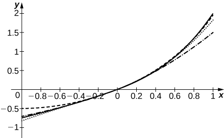
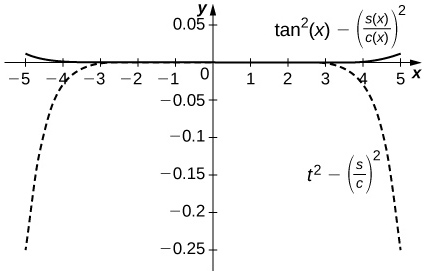
52) [T] Compare \( \dfrac{S_5(x)}{C_4(x)}\) on \( [−1,1]\) to \( \tan x\). Compare this with the Taylor remainder estimate for the approximation of \( \tan x\) by \( x+\dfrac{x^3}{3}+\dfrac{2x^5}{15}\).

Answer

The difference is on the order of \( 10^{−4}\) on \( [−1,1]\) while the Taylor approximation error is around \( 0.1\) near \( ±1\). The top curve is a plot of \(\tan^2x−\left(\dfrac{S_5(x)}{C_4(x)}\right)^2\) and the lower dashed plot shows \( t^2−\left(\dfrac{S_5}{C_4}\right)^2\).

53) [T] Plot \( e^x−e_4(x)\) where \( e_4(x)=1+x+\dfrac{x^2}{2}+\dfrac{x^3}{6}+\dfrac{x^4}{24}\) on \( [0,2]\). Compare the maximum error with the Taylor remainder estimate.

54) (Taylor approximations and root finding.) Recall that Newton’s method \( x_{n+1}=x_n−\dfrac{f(x_n)}{f'(x_n)}\) approximates solutions of \( f(x)=0\) near the input \( x_0\).

a. If \( f\) and \( g\) are inverse functions, explain why a solution of \( g(x)=a\) is the value \( f(a)\) of \( f\).

b. Let \( p_N(x)\) be the \( N^{\text{th}}\) degree Maclaurin polynomial of \( e^x\). Use Newton’s method to approximate solutions of \( p_N(x)−2=0\) for \( N=4,5,6.\)

c. Explain why the approximate roots of \( p_N(x)−2=0\) are approximate values of \(\ln(2).\)

Answer

a. Answers will vary.
b. The following are the \( x_n\) values after \( 10\) iterations of Newton’s method to approximation a root of \( p_N(x)−2=0\): for \( N=4,x=0.6939...;\) for \( N=5,x=0.6932...;\) for \( N=6,x=0.69315...;.\) (Note: \( \ln(2)=0.69314...\))
c. Answers will vary.

Evaluating Limits using Taylor Series

In exercises 55 - 58, use the fact that if \(\displaystyle q(x)=\sum_{n=1}^∞a_n(x−c)^n\) converges in an interval containing \( c\), then \(\displaystyle \lim_{x→c}q(x)=a_0\) to evaluate each limit using Taylor series.

55) \(\displaystyle \lim_{x→0}\frac{\cos x−1}{x^2}\)

56) \(\displaystyle \lim_{x→0}\frac{\ln(1−x^2)}{x^2}\)

Answer

\( \dfrac{\ln(1−x^2)}{x^2}→−1\)

57) \(\displaystyle \lim_{x→0}\frac{e^{x^2}−x^2−1}{x^4}\)

58) \(\displaystyle \lim_{x→0^+}\frac{\cos(\sqrt{x})−1}{2x}\)

Answer

\(\displaystyle \frac{\cos(\sqrt{x})−1}{2x}≈\frac{(1−\frac{x}{2}+\frac{x^2}{4!}−⋯)−1}{2x}→−\frac{1}{4}\)

10.4: Working with Taylor Series

In the following exercises, use appropriate substitutions to write down the Maclaurin series for the given binomial.

1) \(\displaystyle (1−x)^{1/3}\)

2) \(\displaystyle (1+x^2)^{−1/3}\)

Solution: \(\displaystyle (1+x^2)^{−1/3}=\sum_{n=0}^∞(^{−\frac{1}{3}}_n)x^{2n}\)

3) \(\displaystyle (1−x)^{1.01}\)

4) \(\displaystyle (1−2x)^{2/3}\)

Solution: \(\displaystyle (1−2x)^{2/3}=\sum_{n=0}^∞(−1)^n2^n(^{\frac{2}{3}}_n)x^n\)

In the following exercises, use the substitution \(\displaystyle (b+x)^r=(b+a)^r(1+\frac{x−a}{b+a})^r\) in the binomial expansion to find the Taylor series of each function with the given center.

5) (\sqrt{x+2}\) at \(\displaystyle a=0\)

6) \(\displaystyle \sqrt{x^2+2}\) at \(\displaystyle a=0\)

Solution: \(\displaystyle \sqrt{2+x^2}=\sum_{n=0}^∞2^{(1/2)−n}(^{\frac{1}{2}}_n)x^{2n};(∣x^2∣<2)\)

7) \(\displaystyle \sqrt{x+2}\) at \(\displaystyle a=1\)

8) \(\displaystyle \sqrt{2x−x^2}\) at \(\displaystyle a=1\) (Hint: \(\displaystyle 2x−x^2=1−(x−1)^2\))

Solution: \(\displaystyle \sqrt{2x−x^2}=\sqrt{1−(x−1)^2}\) so \(\displaystyle \sqrt{2x−x^2}=\sum_{n=0}^∞(−1)^n(^{\frac{1}{2}}_n)(x−1)^{2n}\)

9) \(\displaystyle (x−8)^{1/3}\) at \(\displaystyle a=9\)

10) \(\displaystyle \sqrt{x}\) at \(\displaystyle a=4\)

Solution: \(\displaystyle \sqrt{x}=2\sqrt{1+\frac{x−4}{4}}\) so \(\displaystyle \sqrt{x}=\sum_{n=0}^∞2^{1−2n}(^{\frac{1}{2}}_n)(x−4)^n\)

11) \(\displaystyle x^{1/3}\) at \(\displaystyle a=27\)

12) \(\displaystyle \sqrt{x}\) at \(\displaystyle x=9\)

Solution: \(\displaystyle \sqrt{x}=\sum_{n=0}^∞3^{1−3n}(^{\frac{1}{2}}_n)(x−9)^n\)

In the following exercises, use the binomial theorem to estimate each number, computing enough terms to obtain an estimate accurate to an error of at most \(\displaystyle 1/1000.\)

13) [T] \(\displaystyle (15)^{1/4}\) using \(\displaystyle (16−x)^{1/4}\)

14) [T] \(\displaystyle (1001)^{1/3}\) using \(\displaystyle (1000+x)^{1/3}\)

Solution: \(\displaystyle 10(1+\frac{x}{1000})^{1/3}=\sum_{n=0}^∞10^{1−3n}(^{\frac{1}{3}}_n)x^n\). Using, for example, a fourth-degree estimate at \(\displaystyle x=1\) gives \(\displaystyle (1001)^{1/3}≈10(1+(^{\frac{1}{3}}_1)10^{−3}+(^{\frac{1}{3}}_2)10^{−6}+(^{\frac{1}{3}}_3)10^{−9}+(^{\frac{1}{3}}_4)10^{−12})=10(1+\frac{1}{3.10^3}−\frac{1}{9.10^6}+\frac{5}{81.10^9}−\frac{10}{243.10^{12}})=10.00333222...\) whereas \(\displaystyle (1001)^{1/3}=10.00332222839093....\) Two terms would suffice for three-digit accuracy.

In the following exercises, use the binomial approximation \(\displaystyle \sqrt{1−x}≈1−\frac{x}{2}−\frac{x^2}{8}−\frac{x^3}{16}−\frac{5x^4}{128}−\frac{7x^5}{256}\) for \(\displaystyle |x|<1\) to approximate each number. Compare this value to the value given by a scientific calculator.

15) [T] \(\displaystyle \frac{1}{\sqrt{2}}\) using \(\displaystyle x=\frac{1}{2}\) in \(\displaystyle (1−x)^{1/2}\)

16) [T] \(\displaystyle \sqrt{5}=5×\frac{1}{\sqrt{5}}\) using \(\displaystyle x=\frac{4}{5}\) in \(\displaystyle (1−x)^{1/2}\)

Solution: The approximation is \(\displaystyle 2.3152\); the CAS value is \(\displaystyle 2.23….\)

17) [T] \(\displaystyle \sqrt{3}=\frac{3}{\sqrt{3}}\) using \(\displaystyle x=\frac{2}{3}\) in \(\displaystyle (1−x)^{1/2}\)

18) [T] \(\displaystyle \sqrt{6}\) using \(\displaystyle x=\frac{5}{6}\) in \(\displaystyle (1−x)^{1/2}\)

Solution: The approximation is \(\displaystyle 2.583…\); the CAS value is \(\displaystyle 2.449….\)

19) Integrate the binomial approximation of \(\displaystyle \sqrt{1−x}\) to find an approximation of \(\displaystyle ∫^x_0\sqrt{1−t}dt\).

20) [T] Recall that the graph of \(\displaystyle \sqrt{1−x^2}\) is an upper semicircle of radius \(\displaystyle 1\). Integrate the binomial approximation of \(\displaystyle \sqrt{1−x^2}\) up to order \(\displaystyle 8\) from \(\displaystyle x=−1\) to \(\displaystyle x=1\) to estimate \(\displaystyle \frac{π}{2}\).

Solution: \(\displaystyle \sqrt{1−x^2}=1−\frac{x^2}{2}−\frac{x^4}{8}−\frac{x^6}{16}−\frac{5x^8}{128}+⋯.\) Thus \(\displaystyle ∫^1_{−1}\sqrt{1−x^2}dx=x−\frac{x^3}{6}−\frac{x^5}{40}−\frac{x^7}{7⋅16}−\frac{5x^9}{9⋅128}+⋯∣^1_{−1}≈2−\frac{1}{3}−\frac{1}{20}−\frac{1}{56}−\frac{10}{9⋅128}+error=1.590...\) whereas \(\displaystyle \frac{π}{2}=1.570...\)

In the following exercises, use the expansion \(\displaystyle (1+x)^{1/3}=1+\frac{1}{3}x−\frac{1}{9}x^2+\frac{5}{81}x^3−\frac{10}{243}x^4+⋯\) to write the first five terms (not necessarily a quartic polynomial) of each expression.

21) \(\displaystyle (1+4x)^{1/3};a=0\)

22) \(\displaystyle (1+4x)^{4/3};a=0\)

Solution: \(\displaystyle (1+x)^{4/3}=(1+x)(1+\frac{1}{3}x−\frac{1}{9}x^2+\frac{5}{81}x^3−\frac{10}{243}x^4+⋯)=1+\frac{4x}{3}+\frac{2x^2}{9}−\frac{4x^3}{81}+\frac{5x^4}{243}+⋯\)

23) \(\displaystyle (3+2x)^{1/3};a=−1\)

24) \(\displaystyle (x^2+6x+10)^{1/3};a=−3\)

Solution: \(\displaystyle (1+(x+3)^2)^{1/3}=1+\frac{1}{3}(x+3)^2−\frac{1}{9}(x+3)^4+\frac{5}{81}(x+3)^6−\frac{10}{243}(x+3)^8+⋯\)

25) Use \(\displaystyle (1+x)^{1/3}=1+\frac{1}{3}x−\frac{1}{9}x^2+\frac{5}{81}x^3−\frac{10}{243}x^4+⋯\) with \(\displaystyle x=1\) to approximate \(\displaystyle 2^{1/3}\).

26) Use the approximation \(\displaystyle (1−x)^{2/3}=1−\frac{2x}{3}−\frac{x^2}{9}−\frac{4x^3}{81}−\frac{7x^4}{243}−\frac{14x^5}{729}+⋯\) for \(\displaystyle |x|<1\) to approximate \(\displaystyle 2^{1/3}=2.2^{−2/3}\).

Solution: Twice the approximation is \(\displaystyle 1.260…\) whereas \(\displaystyle 2^{1/3}=1.2599....\)

27) Find the \(\displaystyle 25th\) derivative of \(\displaystyle f(x)=(1+x^2)^{13}\) at \(\displaystyle x=0\).

28) Find the \(\displaystyle 99\) th derivative of \(\displaystyle f(x)=(1+x^4)^{25}\).

Solution: \(\displaystyle f^{(99)}(0)=0\)

In the following exercises, find the Maclaurin series of each function.

29) \(\displaystyle f(x)=xe^{2x}\)

30) \(\displaystyle f(x)=2^x\)

Solution: \(\displaystyle \sum_{n=0}^∞\frac{(ln(2)x)^n}{n!}\)

31) \(\displaystyle f(x)=\frac{sinx}{x}\)

32) \(\displaystyle f(x)=\frac{sin(\sqrt{x})}{\sqrt{x}},(x>0),\)

Solution: For \(\displaystyle x>0,sin(\sqrt{x})=\sum_{n=0}^∞(−1)^n\frac{x^{(2n+1)/2}}{\sqrt{x}(2n+1)!}=\sum_{n=0}^∞(−1)^n\frac{x^n}{(2n+1)!}\).

33) \(\displaystyle f(x)=sin(x^2)\)

34) \(\displaystyle f(x)=e^{x^3}\)

Solution: \(\displaystyle e^{x^3}=\sum_{n=0}^∞\frac{x^{3n}}{n!}\)

35) \(\displaystyle f(x)=cos^2x\) using the identity \(\displaystyle cos^2x=\frac{1}{2}+\frac{1}{2}cos(2x)\)

36) \(\displaystyle f(x)=sin^2x\) using the identity \(\displaystyle sin^2x=\frac{1}{2}−\frac{1}{2}cos(2x)\)

Solution: \(\displaystyle sin^2x=−\sum_{k=1}^∞\frac{(−1)^k2^{2k−1}x^{2k}}{(2k)!}\)

In the following exercises, find the Maclaurin series of \(\displaystyle F(x)=∫^x_0f(t)dt\) by integrating the Maclaurin series of \(\displaystyle f\) term by term. If \(\displaystyle f\) is not strictly defined at zero, you may substitute the value of the Maclaurin series at zero.

37) \(\displaystyle F(x)=∫^x_0e^{−t^2}dt;f(t)=e^{−t^2}=\sum_{n=0}^∞(−1)^n\frac{t^{2n}}{n!}\)

38) \(\displaystyle F(x)=tan^{−1}x;f(t)=\frac{1}{1+t^2}=\sum_{n=0}^∞(−1)^nt^{2n}\)

Solution: \(\displaystyle tan^{−1}x=\sum_{k=0}^∞\frac{(−1)^kx^{2k+1}}{2k+1}\)

39) \(\displaystyle F(x)=tanh^{−1}x;f(t)=\frac{1}{1−t^2}=\sum_{n=0}^∞t^{2n}\)

40) \(\displaystyle F(x)=sin^{−1}x;f(t)=\frac{1}{\sqrt{1−t^2}}=\sum_{k=0}^∞(^{\frac{1}{2}}_k)\frac{t^{2k}}{k!}\)

Solution: \(\displaystyle sin^{−1}x=\sum_{n=0}^∞(^{\frac{1}{2}}_n)\frac{x^{2n+1}}{(2n+1)n!}\)

41) \(\displaystyle F(x)=∫^x_0\frac{sint}{t}dt;f(t)=\frac{sint}{t}=\sum_{n=0}^∞(−1)^n\frac{t^{2n}}{(2n+1)!}\)

42) \(\displaystyle F(x)=∫^x_0cos(\sqrt{t})dt;f(t)=\sum_{n=0}^∞(−1)^n\frac{x^n}{(2n)!}\)

Solution: \(\displaystyle F(x)=\sum_{n=0}^∞(−1)^n\frac{x^{n+1}}{(n+1)(2n)!}\)

43) \(\displaystyle F(x)=∫^x_0\frac{1−cost}{t^2}dt;f(t)=\frac{1−cost}{t^2}=\sum_{n=0}^∞(−1)^n\frac{t^{2n}}{(2n+2)!}\)

44) \(\displaystyle F(x)=∫^x_0\frac{ln(1+t)}{t}dt;f(t)=\sum_{n=0}^∞(−1)^n\frac{t^n}{n+1}\)

Solution: \(\displaystyle F(x)=\sum_{n=1}^∞(−1)^{n+1}\frac{x^n}{n^2}\)

In the following exercises, compute at least the first three nonzero terms (not necessarily a quadratic polynomial) of the Maclaurin series of \(\displaystyle f\).

45) \(\displaystyle f(x)=sin(x+\frac{π}{4})=sinxcos(\frac{π}{4})+cosxsin(\frac{π}{4})\)

46) \(\displaystyle f(x)=tanx\)

Solution: \(\displaystyle x+\frac{x^3}{3}+\frac{2x^5}{15}+⋯\)

47) \(\displaystyle f(x)=ln(cosx)\)

48) \(\displaystyle f(x)=e^xcosx\)

Solution: \(\displaystyle 1+x−\frac{x^3}{3}−\frac{x^4}{6}+⋯\)

49) \(\displaystyle f(x)=e^{sinx}\)

50) \(\displaystyle f(x)=sec^2x\)

Solution: \(\displaystyle 1+x^2+\frac{2x^4}{3}+\frac{17x^6}{45}+⋯\)

51) \(\displaystyle f(x)=tanhx\)

52) \(\displaystyle f(x)=\frac{tan\sqrt{x}}{\sqrt{x}}\) (see expansion for \(\displaystyle tanx\))

Solution: Using the expansion for \(\displaystyle tanx\) gives \(\displaystyle 1+\frac{x}{3}+\frac{2x^2}{15}\).

In the following exercises, find the radius of convergence of the Maclaurin series of each function.

53) \(\displaystyle ln(1+x)\)

54) \(\displaystyle \frac{1}{1+x^2}\)

Solution: \(\displaystyle \frac{1}{1+x^2}=\sum_{n=0}^∞(−1)^nx^{2n}\) so \(\displaystyle R=1\) by the ratio test.

55) \(\displaystyle tan^{−1}x\)

56) \(\displaystyle ln(1+x^2)\)

Solution: \(\displaystyle ln(1+x^2)=\sum_{n=1}^∞\frac{(−1)^{n−1}}{n}x^{2n}\) so \(\displaystyle R=1\) by the ratio test.

57) Find the Maclaurin series of \(\displaystyle sinhx=\frac{e^x−e^{−x}}{2}\).

58) Find the Maclaurin series of \(\displaystyle coshx=\frac{e^x+e^{−x}}{2}\).

Solution: Add series of \(\displaystyle e^x\) and \(\displaystyle e^{−x}\) term by term. Odd terms cancel and \(\displaystyle coshx=\sum_{n=0}^∞\frac{x^{2n}}{(2n)!}\).

59) Differentiate term by term the Maclaurin series of \(\displaystyle sinhx\) and compare the result with the Maclaurin series of \(\displaystyle coshx\).

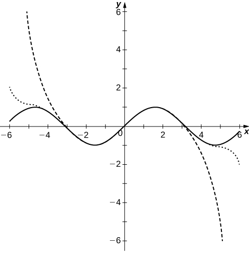
60) [T] Let \(\displaystyle S_n(x)=\sum_{k=0}^n(−1)^k\frac{x^{2k+1}}{(2k+1)!}\) and \(\displaystyle C_n(x)=\sum_{n=0}^n(−1)^k\frac{x^{2k}}{(2k)!}\) denote the respective Maclaurin polynomials of degree \(\displaystyle 2n+1\) of \(\displaystyle sinx\) and degree \(\displaystyle 2n\) of \(\displaystyle cosx\). Plot the errors \(\displaystyle \frac{S_n(x)}{C_n(x)}−tanx\) for \(\displaystyle n=1,..,5\) and compare them to \(\displaystyle x+\frac{x^3}{3}+\frac{2x^5}{15}+\frac{17x^7}{315}−tanx\) on \(\displaystyle (−\frac{π}{4},\frac{π}{4})\).

Solution: The ratio \(\displaystyle \frac{S_n(x)}{C_n(x)}\) approximates \(\displaystyle tanx\) better than does \(\displaystyle p_7(x)=x+\frac{x^3}{3}+\frac{2x^5}{15}+\frac{17x^7}{315}\) for \(\displaystyle N≥3\). The dashed curves are \(\displaystyle \frac{S_n}{C_n}−tan\) for \(\displaystyle n=1,2\). The dotted curve corresponds to \(\displaystyle n=3\), and the dash-dotted curve corresponds to \(\displaystyle n=4\). The solid curve is \(\displaystyle p_7−tanx\).

61) Use the identity \(\displaystyle 2sinxcosx=sin(2x)\) to find the power series expansion of \(\displaystyle sin^2x\) at \(\displaystyle x=0\). (Hint: Integrate the Maclaurin series of \(\displaystyle sin(2x)\) term by term.)

62) If \(\displaystyle y=\sum_{n=0}^∞a_nx^n\), find the power series expansions of \(\displaystyle xy′\) and \(\displaystyle x^2y''\).

Solution: By the term-by-term differentiation theorem, \(\displaystyle y′=\sum_{n=1}^∞na_nx^{n−1}\) so \(\displaystyle y′=\sum_{n=1}^∞na_nx^{n−1}xy′=\sum_{n=1}^∞na_nx^n\), whereas \(\displaystyle y′=\sum_{n=2}^∞n(n−1)a_nx^{n−2}\) so \(\displaystyle xy''=\sum_{n=2}^∞n(n−1)a_nx^n\).

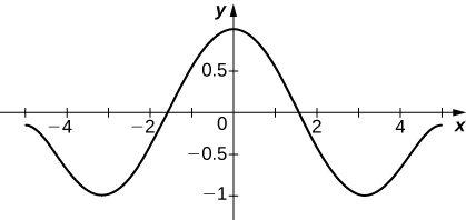
63) [T] Suppose that \(\displaystyle y=\sum_{k=0}^∞a^kx^k\) satisfies \(\displaystyle y′=−2xy\) and \(\displaystyle y(0)=0\). Show that \(\displaystyle a_{2k+1}=0\) for all \(\displaystyle k\) and that \(\displaystyle a_{2k+2}=\frac{−a_{2k}}{k+1}\). Plot the partial sum \(\displaystyle S_{20}\) of \(\displaystyle y\) on the interval \(\displaystyle [−4,4]\).

64) [T] Suppose that a set of standardized test scores is normally distributed with mean \(\displaystyle μ=100\) and standard deviation \(\displaystyle σ=10\). Set up an integral that represents the probability that a test score will be between \(\displaystyle 90\) and \(\displaystyle 110\) and use the integral of the degree \(\displaystyle 10\) Maclaurin polynomial of \(\displaystyle \frac{1}{\sqrt{2π}}e^{−x^2/2}\) to estimate this probability.

Solution: The probability is \(\displaystyle p=\frac{1}{\sqrt{2π}}∫^{(b−μ)/σ}_{(a−μ)/σ}e^{−x^2/2}dx\) where \(\displaystyle a=90\) and \(\displaystyle b=100\), that is, \(\displaystyle p=\frac{1}{\sqrt{2π}}∫^1_{−1}e^{−x^2/2}dx=\frac{1}{\sqrt{2π}}∫^1_{−1}\sum_{n=0}^5(−1)^n\frac{x^{2n}}{2^nn!}dx=\frac{2}{\sqrt{2π}}\sum_{n=0}^5(−1)^n\frac{1}{(2n+1)2^nn!}≈0.6827.\)

65) [T] Suppose that a set of standardized test scores is normally distributed with mean \(\displaystyle μ=100\) and standard deviation \(\displaystyle σ=10\). Set up an integral that represents the probability that a test score will be between \(\displaystyle 70\) and \(\displaystyle 130\) and use the integral of the degree \(\displaystyle 50\) Maclaurin polynomial of \(\displaystyle \frac{1}{\sqrt{2π}}e^{−x^2/2}\) to estimate this probability.

66) [T] Suppose that \(\displaystyle \sum_{n=0}^∞a_nx^n\) converges to a function \(\displaystyle f(x)\) such that \(\displaystyle f(0)=1,f′(0)=0\), and \(\displaystyle f''(x)=−f(x)\). Find a formula for \(\displaystyle a_n\) and plot the partial sum \(\displaystyle S_N\) for \(\displaystyle N=20\) on \(\displaystyle [−5,5].\)

Solution: As in the previous problem one obtains \(\displaystyle a_n=0\) if \(\displaystyle n\) is odd and \(\displaystyle a_n=−(n+2)(n+1)a_{n+2}\) if \(\displaystyle n\) is even, so \(\displaystyle a_0=1\) leads to \(\displaystyle a_{2n}=\frac{(−1)^n}{(2n)!}\).

67) [T] Suppose that \(\displaystyle \sum_{n=0}^∞a_nx^n\) converges to a function \(\displaystyle f(x)\) such that \(\displaystyle f(0)=0,f′(0)=1\), and \(\displaystyle f''(x)=−f(x)\). Find a formula for an and plot the partial sum \(\displaystyle S_N\) for \(\displaystyle N=10\) on \(\displaystyle [−5,5]\).

68) Suppose that \(\displaystyle \sum_{n=0}^∞a_nx^n\) converges to a function \(\displaystyle y\) such that \(\displaystyle y''−y′+y=0\) where \(\displaystyle y(0)=1\) and \(\displaystyle y'(0)=0.\) Find a formula that relates \(\displaystyle a_{n+2},a_{n+1},\) and an and compute \(\displaystyle a_0,...,a_5\).

Solution: \(\displaystyle y''=\sum_{n=0}^∞(n+2)(n+1)a_{n+2}x^n\) and \(\displaystyle y′=\sum_{n=0}^∞(n+1)a_{n+1}x^n\) so \(\displaystyle y''−y′+y=0\) implies that \(\displaystyle (n+2)(n+1)a_{n+2}−(n+1)a_{n+1}+a_n=0\) or \(\displaystyle a_n=\frac{a_{n−1}}{n}−\frac{a_{n−2}}{n(n−1)}\) for all \(\displaystyle n⋅y(0)=a_0=1\) and \(\displaystyle y′(0)=a_1=0,\) so \(\displaystyle a_2=\frac{1}{2},a_3=\frac{1}{6},a_4=0\), and \(\displaystyle a_5=−\frac{1}{120}\).

69) Suppose that \(\displaystyle \sum_{n=0}^∞a_nx^n\) converges to a function \(\displaystyle y\) such that \(\displaystyle y''−y′+y=0\) where \(\displaystyle y(0)=0\) and \(\displaystyle y′(0)=1\). Find a formula that relates \(\displaystyle a_{n+2},a_{n+1}\), and an and compute \(\displaystyle a_1,...,a_5\).

The error in approximating the integral \(\displaystyle ∫^b_af(t)dt\) by that of a Taylor approximation \(\displaystyle ∫^b_aPn(t)dt\) is at most \(\displaystyle ∫^b_aR_n(t)dt\). In the following exercises, the Taylor remainder estimate \(\displaystyle R_n≤\frac{M}{(n+1)!}|x−a|^{n+1}\) guarantees that the integral of the Taylor polynomial of the given order approximates the integral of \(\displaystyle f\) with an error less than \(\displaystyle \frac{1}{10}\).

a. Evaluate the integral of the appropriate Taylor polynomial and verify that it approximates the CAS value with an error less than \(\displaystyle \frac{1}{100}\).

b. Compare the accuracy of the polynomial integral estimate with the remainder estimate.

70) [T] \(\displaystyle ∫^π_0\frac{sint}{t}dt;P_s=1−\frac{x^2}{3!}+\frac{x^4}{5!}−\frac{x^6}{7!}+\frac{x^8}{9!}\) (You may assume that the absolute value of the ninth derivative of \(\displaystyle \frac{sint}{t}\) is bounded by \(\displaystyle 0.1\).)

Solution: a. (Proof) b. We have \(\displaystyle R_s≤\frac{0.1}{(9)!}π^9≈0.0082<0.01.\) We have \(\displaystyle ∫^π_0(1−\frac{x^2}{3!}+\frac{x^4}{5!}−\frac{x^6}{7!}+\frac{x^8}{9!})dx=π−\frac{π^3}{3⋅3!}+\frac{π^5}{5⋅5!}−\frac{π^7}{7⋅7!}+\frac{π^9}{9⋅9!}=1.852...,\) whereas \(\displaystyle ∫^π_0\frac{sint}{t}dt=1.85194...\), so the actual error is approximately \(\displaystyle 0.00006.\)

71) [T] \(\displaystyle ∫^2_0e^{−x^2}dx;p_{11}=1−x^2+\frac{x^4}{2}−\frac{x^6}{3!}+⋯−\frac{x^{22}}{11!}\) (You may assume that the absolute value of the \(\displaystyle 23rd\) derivative of \(\displaystyle e^{−x^2}\) is less than \(\displaystyle 2×10^{14}\).)

The following exercises deal with Fresnel integrals.

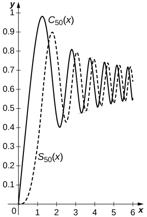
72) The Fresnel integrals are defined by \(\displaystyle C(x)=∫^x_0cos(t^2)dt\) and \(\displaystyle S(x)=∫^x_0sin(t^2)dt\). Compute the power series of \(\displaystyle C(x)\) and \(\displaystyle S(x)\) and plot the sums \(\displaystyle C_N(x)\) and \(\displaystyle S_N(x)\) of the first \(\displaystyle N=50\) nonzero terms on \(\displaystyle [0,2π]\).

Solution: Since \(\displaystyle cos(t^2)=\sum_{n=0}^∞(−1)^n\frac{t^{4n}}{(2n)!}\) and \(\displaystyle sin(t^2)=\sum_{n=0}^∞(−1)^n\frac{t^{4n+2}}{(2n+1)!}\), one has \(\displaystyle S(x)=_sum_{n=0}^∞(−1)^n\frac{x^{4n+3}}{(4n+3)(2n+1)!}\) and \(\displaystyle C(x)=\sum_{n=0}^∞(−1)^n\frac{x^{4n+1}}{(4n+1)(2n)!}\). The sums of the first \(\displaystyle 50\) nonzero terms are plotted below with \(\displaystyle C_{50}(x)\) the solid curve and \(\displaystyle S_{50}(x)\) the dashed curve.

73) [T] The Fresnel integrals are used in design applications for roadways and railways and other applications because of the curvature properties of the curve with coordinates \(\displaystyle (C(t),S(t))\). Plot the curve \(\displaystyle (C_{50},S_{50})\) for \(\displaystyle 0≤t≤2π\), the coordinates of which were computed in the previous exercise.

74) Estimate \(\displaystyle ∫^{1/4}_0\sqrt{x−x^2}dx\) by approximating \(\displaystyle \sqrt{1−x}\) using the binomial approximation \(\displaystyle 1−\frac{x}{2}−\frac{x^2}{8}−\frac{x^3}{16}−\frac{5x^4}{2128}−\frac{7x^5}{256}\).

Solution: \(\displaystyle ∫^{1/4}_0\sqrt{x}(1−\frac{x}{2}−\frac{x^2}{8}−\frac{x^3}{16}−\frac{5x^4}{128}−\frac{7x^5}{256})dx =\frac{2}{3}2^{−3}−\frac{1}{2}\frac{2}{5}2^{−5}−\frac{1}{8}\frac{2}{7}2^{−7}−\frac{1}{16}\frac{2}{9}2^{−9}−\frac{5}{128}\frac{2}{11}2^{−11}−\frac{7}{256}\frac{2}{13}2^{−13}=0.0767732...\) whereas \(\displaystyle ∫^{1/4}_0\sqrt{x−x^2}dx=0.076773.\)

75) [T] Use Newton’s approximation of the binomial \(\displaystyle \sqrt{1−x^2}\) to approximate \(\displaystyle π\) as follows. The circle centered at \(\displaystyle (\frac{1}{2},0)\) with radius \(\displaystyle \frac{1}{2}\) has upper semicircle \(\displaystyle y=\sqrt{x}\sqrt{1−x}\). The sector of this circle bounded by the \(\displaystyle x\)-axis between \(\displaystyle x=0\) and \(\displaystyle x=\frac{1}{2}\) and by the line joining \(\displaystyle (\frac{1}{4},\frac{\sqrt{3}}{4})\) corresponds to \(\displaystyle \frac{1}{6}\) of the circle and has area \(\displaystyle \frac{π}{24}\). This sector is the union of a right triangle with height \(\displaystyle \frac{\sqrt{3}}{4}\) and base \(\displaystyle \frac{1}{4}\) and the region below the graph between \(\displaystyle x=0\) and \(\displaystyle x=\frac{1}{4}\). To find the area of this region you can write \(\displaystyle y=\sqrt{x}\sqrt{1−x}=\sqrt{x}×(\text{binomial expansion of} \sqrt{1−x})\) and integrate term by term. Use this approach with the binomial approximation from the previous exercise to estimate \(\displaystyle π\).

76) Use the approximation \(\displaystyle T≈2π\sqrt{\frac{L}{g}}(1+\frac{k^2}{4})\) to approximate the period of a pendulum having length \(\displaystyle 10\) meters and maximum angle \(\displaystyle θ_{max}=\frac{π}{6}\) where \(\displaystyle k=sin(\frac{θ_{max}}{2})\). Compare this with the small angle estimate \(\displaystyle T≈2π\sqrt{\frac{L}{g}}\).

Solution: \(\displaystyle T≈2π\sqrt{\frac{10}{9.8}}(1+\frac{sin^2(θ/12)}{4})≈6.453\) seconds. The small angle estimate is \(\displaystyle T≈2π\sqrt{\frac{10}{9.8}≈6.347}\). The relative error is around \(\displaystyle 2\) percent.

77) Suppose that a pendulum is to have a period of \(\displaystyle 2\) seconds and a maximum angle of \(\displaystyle θ_{max}=\frac{π}{6}\). Use \(\displaystyle T≈2π\sqrt{\frac{L}{g}}(1+\frac{k^2}{4})\) to approximate the desired length of the pendulum. What length is predicted by the small angle estimate \(\displaystyle T≈2π\sqrt{\frac{L}{g}}\)?

78) Evaluate \(\displaystyle ∫^{π/2}_0sin^4θdθ\) in the approximation \(\displaystyle T=4\sqrt{\frac{L}{g}}∫^{π/2}_0(1+\frac{1}{2}k^2sin^2θ+\frac{3}{8}k^4sin^4θ+⋯)dθ\) to obtain an improved estimate for \(\displaystyle T\).

Solution: \(\displaystyle ∫^{π/2}_0sin^4θdθ=\frac{3π}{16}.\) Hence \(\displaystyle T≈2π\sqrt{\frac{L}{g}}(1+\frac{k^2}{4}+\frac{9}{256}k^4).\)

79) [T] An equivalent formula for the period of a pendulum with amplitude \(\displaystyle θ_max\) is \(\displaystyle T(θ_{max})=2\sqrt{2}\sqrt{\frac{L}{g}}∫^{θ_{max}}_0\frac{dθ}{\sqrt{cosθ}−cos(θ_{max})}\) where \(\displaystyle L\) is the pendulum length and \(\displaystyle g\) is the gravitational acceleration constant. When \(\displaystyle θ_{max}=\frac{π}{3}\) we get \(\displaystyle \frac{1}{\sqrt{cost−1/2}}≈\sqrt{2}(1+\frac{t^2}{2}+\frac{t^4}{3}+\frac{181t^6}{720})\). Integrate this approximation to estimate \(\displaystyle T(\frac{π}{3})\) in terms of \(\displaystyle L\) and \(\displaystyle g\). Assuming \(\displaystyle g=9.806\) meters per second squared, find an approximate length \(\displaystyle L\) such that \(\displaystyle T(\frac{π}{3})=2\) seconds.

Chapter Review Exercise

True or False? In the following exercises, justify your answer with a proof or a counterexample.

1) If the radius of convergence for a power series \(\displaystyle \sum_{n=0}^∞a_nx^n\) is \(\displaystyle 5\), then the radius of convergence for the series \(\displaystyle \sum_{n=1}^∞na_nx^{n−1}\) is also \(\displaystyle 5\).

Solution: True

2) Power series can be used to show that the derivative of \(\displaystyle e^x\) is \(\displaystyle e^x\). (Hint: Recall that \(\displaystyle e^x=\sum_{n=0}^∞\frac{1}{n!}x^n.\))

3) For small values of \(\displaystyle x,sinx≈x.\)

Solution: True

4) The radius of convergence for the Maclaurin series of \(\displaystyle f(x)=3^x\) is \(\displaystyle 3\).

In the following exercises, find the radius of convergence and the interval of convergence for the given series.

5) \(\displaystyle \sum_{n=0}^∞n^2(x−1)^n\)

Solution: ROC: \(\displaystyle 1\); IOC: \(\displaystyle (0,2)\)

6) \(\displaystyle \sum_{n=0}^∞\frac{x^n}{n^n}\)

7) \(\displaystyle \sum_{n=0}^∞\frac{3nx^n}{12^n}\)

Solution: ROC: \(\displaystyle 12;\) IOC: \(\displaystyle (−16,8)\)

8) \(\displaystyle \sum_{n=0}^∞\frac{2^n}{e^n}(x−e)^n\)

In the following exercises, find the power series representation for the given function. Determine the radius of convergence and the interval of convergence for that series.

9) \(\displaystyle f(x)=\frac{x^2}{x+3}\)

Solution: \(\displaystyle \sum_{n=0}^∞\frac{(−1)^n}{3^{n+1}}x^n;\) ROC: \(\displaystyle 3\); IOC: \(\displaystyle (−3,3)\)

10) \(\displaystyle f(x)=\frac{8x+2}{2x^2−3x+1}\)

In the following exercises, find the power series for the given function using term-by-term differentiation or integration.

11) \(\displaystyle f(x)=tan^{−1}(2x)\)

Solution: integration: \(\displaystyle \sum_{n=0}^∞\frac{(−1)^n}{2n+1}(2x)^{2n+1}\)

12) \(\displaystyle f(x)=\frac{x}{(2+x^2)^2}\)

In the following exercises, evaluate the Taylor series expansion of degree four for the given function at the specified point. What is the error in the approximation?

13) \(\displaystyle f(x)=x^3−2x^2+4,a=−3\)

Solution: \(\displaystyle p_4(x)=(x+3)^3−11(x+3)^2+39(x+3)−41;\) exact

14) \(\displaystyle f(x)=e^{1/(4x)},a=4\)

In the following exercises, find the Maclaurin series for the given function.

15) \(\displaystyle f(x)=cos(3x)\)

Solution: \(\displaystyle \sum_{n=0}^∞\frac{(−1)^n(3x)^{2n}}{2n!}\)

16) \(\displaystyle f(x)=ln(x+1)\)

In the following exercises, find the Taylor series at the given value.

17) \(\displaystyle f(x)=sinx,a=\frac{π}{2}\)

Solution: \(\displaystyle \sum_{n=0}^∞\frac{(−1)^n}{(2n)!}(x−\frac{π}{2})^{2n}\)

18) \(\displaystyle f(x)=\frac{3}{x},a=1\)

In the following exercises, find the Maclaurin series for the given function.

19) \(\displaystyle f(x)=e^{−x^2}−1\)

Solution: \(\displaystyle \sum_{n=1}^∞\frac{(−1)^n}{n!}x^{2n}\)

20) \(\displaystyle f(x)=cosx−xsinx\)

In the following exercises, find the Maclaurin series for \(\displaystyle F(x)=∫^x_0f(t)dt\) by integrating the Maclaurin series of \(\displaystyle f(x)\) term by term.

21) \(\displaystyle f(x)=\frac{sinx}{x}\)

Solution: \(\displaystyle F(x)=\sum_{n=0}^∞\frac{(−1)^n}{(2n+1)(2n+1)!}x^{2n+1}\)

22) \(\displaystyle f(x)=1−e^x\)

23) Use power series to prove Euler’s formula: \(\displaystyle e^{ix}=cosx+isinx\)

Solution: Answers may vary.

The following exercises consider problems of annuity payments.

24) For annuities with a present value of \(\displaystyle $1\) million, calculate the annual payouts given over \(\displaystyle 25\) years assuming interest rates of \(\displaystyle 1%,5%\), and \(\displaystyle 10%.\)

25) A lottery winner has an annuity that has a present value of \(\displaystyle $10\) million. What interest rate would they need to live on perpetual annual payments of \(\displaystyle $250,000\)?

Solution: \(\displaystyle 2.5%\)

26) Calculate the necessary present value of an annuity in order to support annual payouts of \(\displaystyle $15,000\) given over \(\displaystyle 25\) years assuming interest rates of \(\displaystyle 1%,5%\),and \(\displaystyle 10%.\)

Contributors and Attributions

• Gilbert Strang (MIT) and Edwin “Jed” Herman (Harvey Mudd) with many contributing authors. This content by OpenStax is licensed with a CC-BY-SA-NC 4.0 license. Download for free at http://cnx.org.