15.E: Multiple Integration (Exercises)

15.1: Double Integrals over Rectangular Regions

In the following exercises, use the midpoint rule with $m = 4$ and $n = 2$ to estimate the volume of the solid bounded by the surface $z = f(x,y)$, the vertical planes $x = 1$, $x = 2$, $y = 1$, and $y = 2$, and the horizontal plane $x = 0$.

$f(x,y) = 4x + 2y + 8xy$

[Hide Solution]

27.

$f(x,y) = 16x^2 + \frac{y}{2}$

In the following exercises, estimate the volume of the solid under the surface $z = f(x,y)$ and above the rectangular region R by using a Riemann sum with $m = n = 2$ and the sample points to be the lower left corners of the subrectangles of the partition.

$f(x,y) = sin \space x - cos \space y$, $R = [0, \pi] \times [0, \pi]$

[Hide Solution]

0.

$f(x,y) = cos \space x + cos \space y$, $R = [0, \pi] \times [0, \frac{\pi}{2}]$

Use the midpoint rule with $m = n = 2$ to estimate $\iint_R f(x,y) dA$, where the values of the function f on $R = [8,10] \times [9,11]$ are given in the following table.

	y
x	9	9.5	10	10.5	11
8	9.8	5	6.7	5	5.6
8.5	9.4	4.5	8	5.4	3.4
9	8.7	4.6	6	5.5	3.4
9.5	6.7	6	4.5	5.4	6.7
10	6.8	6.4	5.5	5.7	6.8

[Hide Solution]

21.3.

The values of the function f on the rectangle $R = [0,2] \times [7,9]$ are given in the following table. Estimate the double integral $\iint_R f(x,y)dA$ by using a Riemann sum with $m = n = 2$. Select the sample points to be the upper right corners of the subsquares of R.

	$y_0 = 7$	$y_1 = 8$	$y_2 = 9$
$x_0 = 0$	10.22	10.21	9.85
$x_1 = 1$	6.73	9.75	9.63
$x_2 = 2$	5.62	7.83	8.21

The depth of a children’s 4-ft by 4-ft swimming pool, measured at 1-ft intervals, is given in the following table.

1. Estimate the volume of water in the swimming pool by using a Riemann sum with $m = n = 2$. Select the sample points using the midpoint rule on $R = [0,4] \times [0,4]$.
2. Find the average depth of the swimming pool.

   	y
   x	0	1	2	3	4
   0	1	1.5	2	2.5	3
   1	1	1.5	2	2.5	3
   2	1	1.5	1.5	2.5	3
   3	1	1	1.5	2	2.5
   4	1	1	1	1.5	2

[Hide Solution]

a. 28 $ft^3$ b. 1.75 ft.

The depth of a 3-ft by 3-ft hole in the ground, measured at 1-ft intervals, is given in the following table.

1. Estimate the volume of the hole by using a Riemann sum with $m = n = 3$ and the sample points to be the upper left corners of the subsquares of $R$.
2. Find the average depth of the hole.

   	y
   x	0	1	2	3
   0	6	6.5	6.4	6
   1	6.5	7	7.5	6.5
   2	6.5	6.7	6.5	6
   3	6	6.5	5	5.6

The level curves $f(X,Y) = K$ of the function f are given in the following graph, where k is a constant.

1. Apply the midpoint rule with $M = N = 2$m=n=2m=n=2 to estimate the double integral $\iint_R f(x,y)dA$, where $R = [0.2,1] \times [0,0.8]$.
2. Estimate the average value of the function f on $R$.

   

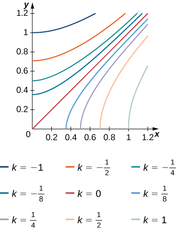
a. 0.112 b. $f_{ave} ≃ 0.175$; here $f(0.4,0.2) ≃ 0.1$, $f(0.2,0.6) ≃− 0.2$, $f(0.8,0.2) ≃ 0.6$, and $f(0.8,0.6) ≃ 0.2$.

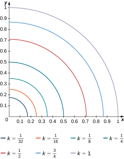
The level curves $f(x,y) = k$ of the function f are given in the following graph, where k is a constant.

1. Apply the midpoint rule with $m = n = 2$ to estimate the double integral $\iint_R f(x,y)dA$, where $R = [0.1,0.5] \times [0.1,0.5]$.
2. Estimate the average value of the function f on $R$.

   

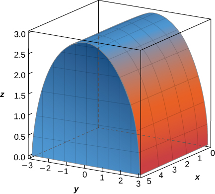
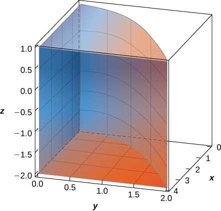
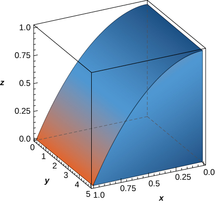
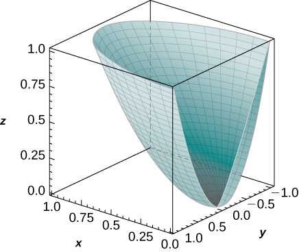
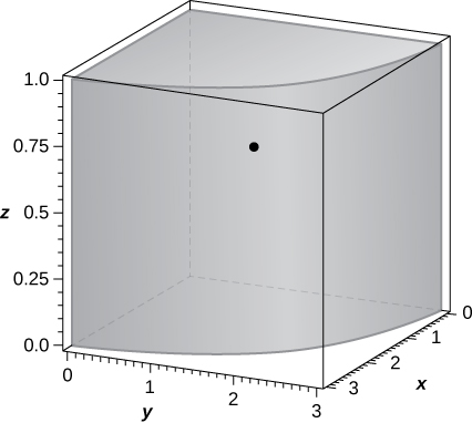
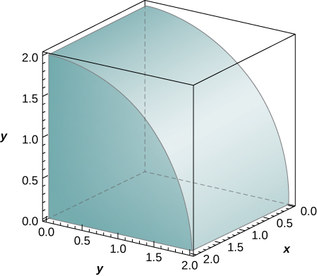
The solid lying under the surface $z = \sqrt{4 - y^2}$ and above the rectangular region$R = [0,2] \times [0,2]$ is illustrated in the following graph. Evaluate the double integral $\iint_Rf(x,y)$, where $f(x,y) = \sqrt{4 - y^2}$ by finding the volume of the corresponding solid.

[Hide Solution]

$2\pi$

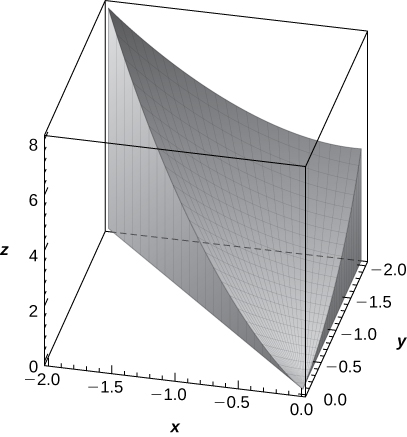
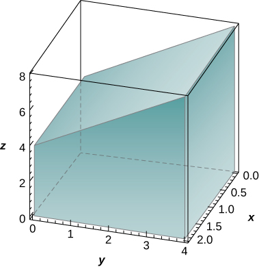
The solid lying under the plane $z = y + 4$ and above the rectangular region $R = [0,2] \times [0,4]$ is illustrated in the following graph. Evaluate the double integral $\iint_R f(x,y)dA$, where $f(x,y) = y + 4$, by finding the volume of the corresponding solid.

In the following exercises, calculate the integrals by interchanging the order of integration.

$$\int_{-1}^1\left(\int_{-2}^2 (2x + 3y + 5)dx \right) \space dy$$

[Hide Solution]

40.

$$\int_0^2\left(\int_0^1 (x + 2e^y + 3)dx \right) \space dy$$

$$\int_1^{27}\left(\int_1^2 (\sqrt[3]{x} + \sqrt[3]{y})dy \right) \space dx$$

[Hide Solution]

$\frac{81}{2} + 39\sqrt[3]{2}$.

$$\int_1^{16}\left(\int_1^8 (\sqrt[4]{x} + 2\sqrt[3]{y})dy \right) \space dx$$

$$\int_{ln \space 2}^{ln \space 3}\left(\int_0^1 e^{x+y}dy \right) \space dx$$

[Hide Solution]

$e - 1$.

$$\int_0^2\left(\int_0^1 3^{x+y}dy \right) \space dx$$

$$\int_1^6\left(\int_2^9 \frac{\sqrt{y}}{y^2}dy \right) \space dx$$

[Hide Solution]

$15 - \frac{10\sqrt{2}}{9}$.

$$\int_1^9 \left(\int_4^2 \frac{\sqrt{x}}{y^2}dy \right) dx$$

In the following exercises, evaluate the iterated integrals by choosing the order of integration.

$$\int_0^{\pi} \int_0^{\pi/2} sin(2x)cos(3y)dx \space dy$$

[Hide Solution]

0.

$$\int_{\pi/12}^{\pi/8}\int_{\pi/4}^{\pi/3} [cot \space x + tan(2y)]dx \space dy$$

$$\int_1^e \int_1^e \left[\frac{1}{x}sin(ln \space x) + \frac{1}{y}cos (ln \space y)\right] dx \space dy$$

[Hide Solution]

$(e − 1)(1 + sin1 − cos1)$

$$\int_1^e \int_1^e \frac{sin(ln \space x)cos (ln \space y)}{xy} dx \space dy$$

$$\int_1^2 \int_1^2 \left(\frac{ln \space y}{x} + \frac{x}{2y + 1}\right) dy \space dx$$

[Hide solution]

$\frac{3}{4}ln \left(\frac{5}{3}\right) + 2b \space ln^2 2 - ln \space 2$

$$\int_1^e \int_1^2 x^2 ln(x) dy \space dx$$

$$\int_1^{\sqrt{3}} \int_1^2 y \space arctan \left(\frac{1}{x}\right) dy \space dx$$

[Hide Solution]

$\frac{1}{8}[(2\sqrt{3} - 3) \pi + 6 \space ln \space 2]$.

$$\int_0^1 \int_0^{1/2} (arcsin \space x + arcsin \space y) dy \space dx$$

$$\int_0^1 \int_0^2 xe^{x+4y} dy \space dx$$

[Hide Solution]

$\frac{1}{4}e^4 (e^4 - 1)$.

$$\int_1^2 \int_0^1 xe^{x-y} dy \space dx$$

$$\int_1^e \int_1^e \left(\frac{ln \space y}{\sqrt{y}} + \frac{ln \space x}{\sqrt{x}}\right) dy \space dx$$

[Hide Solution]

$4(e - 1)(2 - \sqrt{e})$.

$$\int_1^e \int_1^e \left(\frac{x \space ln \space y}{\sqrt{y}} + \frac{y \space ln \space x}{\sqrt{x}}\right) dy \space dx$$

$$\int_0^1 \int_1^2 \left(\frac{x}{x^2 + y^2} \right) dy \space dx$$

[Hide Solution]

$-\frac{\pi}{4} + ln \left(\frac{5}{4}\right) - \frac{1}{2} ln \space 2 + arctan \space 2$.

$$\int_0^1 \int_1^2 \frac{y}{x + y^2} dy \space dx$$

In the following exercises, find the average value of the function over the given rectangles.

$f(x,y) = −x +2y$, $R = [0,1] \times [0,1]$

[Hide Solution]

$\frac{1}{2}$.

$f(x,y) = x^4 + 2y^3$, $R = [1,2] \times [2,3]$

$f(x,y) = sinh \space x + sinh \space y$, $R = [0,1] \times [0,2]$

[Hide solution]

$\frac{1}{2}(2 \space cosh \space 1 + cosh \space 2 - 3)$.

$f(x,y) = arctan(xy)$, $R = [0,1] \times [0,1]$

Let f and g be two continuous functions such that $0 \leq m_1 \leq f(x) \leq M_1$ for any $x ∈ [a,b]$ and $0 \leq m_2 \leq g(y) \leq M_2$ for any$y ∈ [c,d]$. Show that the following inequality is true:

$$m_1m_2(b-a)(c-d) \leq \int_a^b \int_c^d f(x) g(y) dy dx \leq M_1M_2 (b-a)(c-d).$$

In the following exercises, use property v. of double integrals and the answer from the preceding exercise to show that the following inequalities are true.

$\frac{1}{e^2} \leq \iint_R e^{-x^2 - y^2} \space dA \leq 1$, where $R = [0,1] \times [0,1]$

$\frac{\pi^2}{144} \leq \iint_R sin \space x \space cos y \space dA \leq \frac{\pi^2}{48}$, where $R = \left[ \frac{\pi}{6}, \frac{\pi}{3}\right] \times \left[ \frac{\pi}{6}, \frac{\pi}{3}\right]$

$0 \leq \iint_R e^{-y}\space cos x \space dA \leq \frac{\pi}{2}$, where $R = \left[0, \frac{\pi}{2}\right] \times \left[0, \frac{\pi}{2}\right]$

$0 \leq \iint_R (ln \space x)(ln \space y) dA \leq (e - 1)^2$, where $R = [1, e] \times [1, e]$

Let f and g be two continuous functions such that $0 \leq m_1 \leq f(x) \leq M_1$ for any $x ∈ [a,b]$ and $0 \leq m_2 \leq g(y) \leq M_2$ for any $y ∈ [c,d]$. Show that the following inequality is true:

$(m_1 + m_2) (b - a)(c - d) \leq \int_a^b \int_c^d |f(x) + g(y)| \space dy \space dx \leq (M_1 + M_2)(b - a)(c - d)$.

In the following exercises, use property v. of double integrals and the answer from the preceding exercise to show that the following inequalities are true.

$\frac{2}{e} \leq \iint_R (e^{-x^2} + e^{-y^2}) dA \leq 2$, where $R = [0,1] \times [0,1]$

$\frac{\pi^2}{36}\iint_R (sin \space x + cos \space y)dA \leq \frac{\pi^2 \sqrt{3}}{36}$, where $R = [\frac{\pi}{6}, \frac{\pi}{3}] \times [\frac{\pi}{6}, \frac{\pi}{3}]$

$\frac{\pi}{2}e^{-\pi/2} \leq \iint_R (cos \space x + e^{-y})dA \leq \pi$, where $R = [0, \frac{\pi}{2}] \times [0, \frac{\pi}{2}]$

$\frac{1}{e} \leq \iint_R (e^{-y} - ln \space x) dA \leq 2$, where $R = [0, 1] \times [0, 1]$

In the following exercises, the function f is given in terms of double integrals.

1. Determine the explicit form of the function f.
2. Find the volume of the solid under the surface $z = f(x,y)$ and above the region R.
3. Find the average value of the function f on R.
4. Use a computer algebra system (CAS) to plot $z = f(x,y)$ and $z = f_{ave}$ in the same system of coordinates.

[T] $f(x,y) = \int_0^y \int_0^x (xs + yt) ds \space dt$, where $(x,y) \in R = [0,1] \times [0,1]$

[Hide Solution]

a. $f(x,y) = \frac{1}{2} xy (x^2 + y^2)$; b. $V = \int_0^1 \int_0^1 f(x,y) dx \space dy = \frac{1}{8}$; c. $f_{ave} = \frac{1}{8}$;

d.

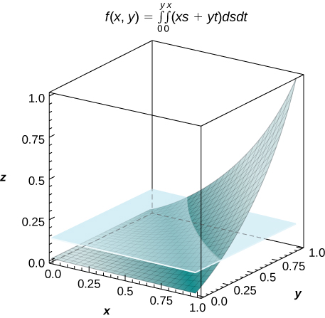
[T] $f(x,y) = \int_0^x \int_0^y [cos \space (s) + cos \space (t)] dt \space ds$, where $(x,y) \in R = [0,3] \times [0,3]$

Show that if f and g are continuous on $[a,b]$ and $[c,d]$, respectively, then

$\int_a^b \int_c^d |f(x) + g(y)| dy \space dx = (d - c) \int_a^b f(x)dx$

$+ \int_a^b \int_c^d g(y)dy \space dx = (b - a) \int_c^d g(y)dy + \int_c^d \int_a^b f(x) dx \space dy$.

Show that $\int_a^b \int_c^d yf(x) + xg(y) dy \space dx = \frac{1}{2} (d^2 - c^2) \left(\int_a^b f(x)dx\right) + \frac{1}{2} (b^2 - a^2) \left(\int_c^d g(y)dy\right)$.

[T] Consider the function $f(x,y) = e^{-x^2-y^2}$, where $(x,y) \in R = [−1,1] \times [−1,1]$.

1. Use the midpoint rule with $m = n = 2,4,..., 10$ to estimate the double integral $I = \iint_R e^{-x^2 - y^2} dA$. Round your answers to the nearest hundredths.
2. For $m = n = 2$, find the average value of f over the region R. Round your answer to the nearest hundredths.
3. Use a CAS to graph in the same coordinate system the solid whose volume is given by $\iint_R e^{-x^2-y^2} dA$ and the plane $z = f_{ave}$.

[Hide Solution]

a. For $m = n = 2$, $I = 4e^{-0.5} \approx 2.43$ b. $f_{ave} = e^{-0.5} \simeq 0.61$;

c.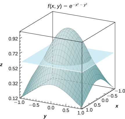

[T] Consider the function $f(x,y) = sin \space (x^2) \space cos \space (y^2)$, where $(x,y \in R = [−1,1] \times [−1,1]$.

1. Use the midpoint rule with $m = n = 2,4,..., 10$ to estimate the double integral $I = \iint_R sin \space (x^2) \space cos \space (y^2) \space dA$. Round your answers to the nearest hundredths.
2. For $m = n = 2$, find the average value of f over the region R. Round your answer to the nearest hundredths.
3. Use a CAS to graph in the same coordinate system the solid whose volume is given by $\iint_R sin \space (x^2) \space cos \space (y^2) \space dA$ and the plane $z = f_{ave}$.

In the following exercises, the functions fnfn are given, where $n \geq 1$ is a natural number.

1. Find the volume of the solids $S_n$ under the surfaces $z = f_n(x,y)$ and above the region R.
2. Determine the limit of the volumes of the solids $S_n$ as n increases without bound.

$f(x,y) = x^n + y^n + xy, \space (x,y) \in R = [0,1] \times [0,1]$

[Hide Solution]

a. $\frac{2}{n + 1} + \frac{1}{4}$ b. $\frac{1}{4}$

$f(x,y) = \frac{1}{x^n} + \frac{1}{y^n}, \space (x,y) \in R = [1,2] \times [1,2]$

Show that the average value of a function f on a rectangular region $R = [a,b] \times [c,d]$ is $f_{ave} \approx \frac{1}{mn} \sum_{i=1}^m \sum_{j=1}^n f(x_{ij}^*,y_{ij}^*)$,where $(x_{ij}^*,y_{ij}^*)$ are the sample points of the partition of R, where $1 \leq i \leq m$ and $1 \leq j \leq n$.

Use the midpoint rule with $m = n$ to show that the average value of a function f on a rectangular region $R = [a,b] \times [c,d]$ is approximated by

$$f_{ave} \approx \frac{1}{n^2} \sum_{i,j =1}^n f \left(\frac{1}{2} (x_{i=1} + x_i), \space \frac{1}{2} (y_{j=1} + y_j)\right).$$

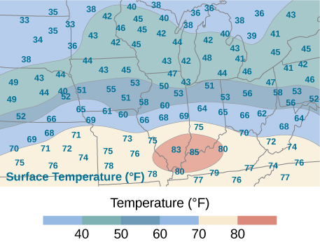
An isotherm map is a chart connecting points having the same temperature at a given time for a given period of time. Use the preceding exercise and apply the midpoint rule with $m = n = 2$ to find the average temperature over the region given in the following figure.

[Hide Solution]

$56.5^{\circ}$ F; here $f(x_1^*,y_1^*) = 71, \space f(x_2^*, y_1^*) = 72, \space f(x_2^*,y_1^*) = 40, \space f(x_2^*,y_2^*) = 43$, where $x_i^*$ and $y_j^*$ are the midpoints of the subintervals of the partitions of [a,b] and [c,d], respectively

15.2: Double Integrals over General Regions

In the following exercises, specify whether the region is of Type I or Type II.

The region $D$ bounded by $y = x^3, \space y = x^3 + 1, \space x = 0,$ and $x = 1$ as given in the following figure.

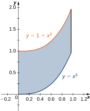
Find the average value of the function $f(x,y) = 3xy$ on the region graphed in the previous exercise.

[Hide Solution]

$\frac{27}{20}$

Find the area of the region $D$ given in the previous exercise.

The region $D$ bounded by $y = sin \space x, \space y = 1 + sin \space x, \space x = 0$, and $x = \frac{\pi}{2}$ as given in the following figure.

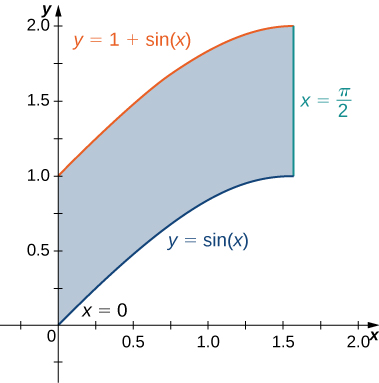
[Hide Solution]

Type I but not Type II

Find the average value of the function $f(x,y) = cos \space x$ on the region graphed in the previous exercise.

Find the area of the region $D$ given in the previous exercise.

[Hide Solution]

$\frac{\pi}{2}$

The region $D$ bounded by $x = y^2 - 1$ and $x = \sqrt{1 - y^2}$ as given in the following figure.

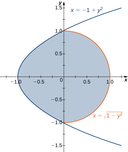
Find the volume of the solid under the graph of the function $f(x,y) = xy + 1$ and above the region in the figure in the previous exercise.

[Hide Solution]

$\frac{1}{6}(8 + 3\pi)$

The region $D$ bounded by $y = 0, \space x = -10 + y,$ and $x = 10 - y$ as given in the following figure.

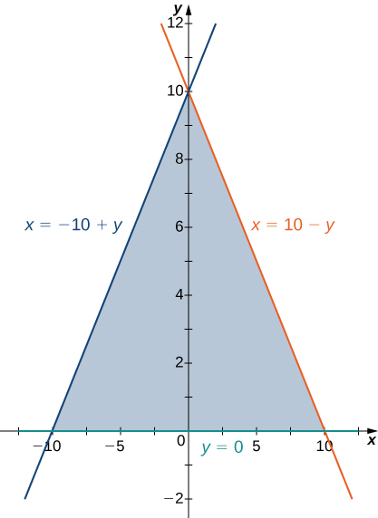
Find the volume of the solid under the graph of the function $f(x,y) = x + y$ and above the region in the figure from the previous exercise.

[Hide Solution]

$\frac{1000}{3}$

The region $D$ bounded by $y = 0, \space x = y - 1, \space x = \frac{\pi}{2}$ as given in the following figure.

The region $D$ bounded by $y = 0$ and $y = x^2 - 1$ as given in the following figure.

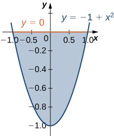
Type I and Type II

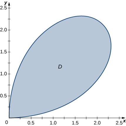
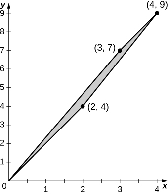
Let $D$ be the region bounded by the curves of equations $y = x, \space y = -x$ and $y = 2 - x^2$. Explain why $D$ is neither of Type I nor II.

Let $D$ be the region bounded by the curves of equations $y = cos \space x$ and $y = 4 - x^2$ and the $x$-axis. Explain why $D$ is neither of Type I nor II.

[Hide Solution]

The region $D$ is not of Type I: it does not lie between two vertical lines and the graphs of two continuous functions $g_1(x)$ and $g_2(x)$. The region D is not of Type II: it does not lie between two horizontal lines and the graphs of two continuous functions $h_1(y)$ and $h_2(y)$.

In the following exercises, evaluate the double integral $\iint_D f(x,y) dA$ over the region $D$.

$f(x,y) = 2x + 4y$ and

$D = \big\{(x,y)|\, 0 \leq x \leq 1, \space x^3 \leq y \leq x^3 + 1 \big\}$

$f(x,y) = 1$ and

$D = \big\{(x,y)| \, 0 \leq x \leq \frac{\pi}{2}, \space \sin x \leq y \leq 1 + \sin x \big\}$

[Hide Solution]

$\frac{\pi}{2}$

$f(x,y) = 2$ and

$D = \big\{(x,y)| \, 0 \leq y \leq 1, \space y - 1 \leq x \leq \arccos y \big\}$

$f(x,y) = xy$ and

$D = \big\{(x,y)| \, -1 \leq y \leq 1, \space y^2 - 1 \leq x \leq \sqrt{1 - y^2} \big\}$

[Hide Solution]

0

$f(x,y) = sin \space y$ and $D$ is the triangular region with vertices $(0,0), \space (0,3)$, and $(3,0)$

$f(x,y) = -x + 1$ and $D$ is the triangular region with vertices $(0,0), \space (0,2)$, and $(2,2)$

[Hide Solution]

$\frac{2}{3}$

Evaluate the iterated integrals.

$$\int_0^3 \int_{2x}^{3x} (x + y^2) dy \space dx$$

$$\int_0^1 \int_{2\sqrt{x}}^{2\sqrt{x}+1} (xy + 1) dy \space dx$$

[Hide Solution]

$\frac{41}{20}$

$$\int_e^{e^2} \int_{ln \space u}^2 (v + ln \space u) dv \space du$$

$$\int_1^2 \int_{-u^2-1}^{-u} (8 uv) dv \space du$$

[Hide Solution]

$-63$

$$\int_0^1 \int_{-\sqrt{1-y^2}}^{\sqrt{1-y^2}} (2x + 4y^3) dx \space dy$$

$$\int_0^1 \int_{-\sqrt{1-4y^2}}^{\sqrt{1-4y^2}} 4dx \space dy$$

[Hide Solution]

$\pi$

Let $D$ be the region bounded by $y = 1 - x^2, \space y = 4 - x^2$, and the $x$- and $y$-axes.

a. Show that

$$\iint_D xdA = \int_0^1 \int_{1-x^2}^{4-x^2} x \space dy \space dx + \int_1^2 \int_0^{4-x^2} x \space dy \space dx$$ by dividing the region $D$ into two regions of Type I.

b. Evaluate the integral $$\iint_D s \space dA.$$

Let $D$ be the region bounded by $y = 1, \space y = x, \space y = ln \space x$, and the $x$-axis.

a. Show that

$$\iint_D y^2 dA = \int_{-1}^0 \int_{-x}^{2-x^2} y^2 dy \space dx + \int_0^1 \int_x^{2-x^2} y^2 dy \space dx$$ by dividing the region $D$ into two regions of Type I, where $D = {(x,y)|y \geq x, y \geq -x, \space y \leq 2-x^2}$.

b. Evaluate the integral $$\iint_D y^2 dA.$$

Let $D$ be the region bounded by $y = x^2$, $y = x + 2$, and $y = -x$.

a. Show that $$\iint_D x \space dA = \int_0^1 \int_{-y}^{\sqrt{y}} x \space dx \space dy + \int_1^2 \int_{y-2}^{\sqrt{y}} x \space dx \space dy$$ by dividing the region $D$ into two regions of Type II, where $D = {(x,y)|y \geq x^2, \space y \geq -x, \space y \leq x + 2}$.

b. Evaluate the integral $$\iint_D x \space dA.$$

[Hide Solution]

a. Answers may vary; b. $\frac{8}{12}$

The region $D$ bounded by $x = 0, y = x^5 + 1$, and $y = 3 - x^2$ is shown in the following figure. Find the area $A(D)$ of the region $D$.

The region $D$ bounded by $y = cos \space x, \space y = 4 \space cos \space x$, and $x = \pm \frac{\pi}{3}$ is shown in the following figure. Find the area $A(D)$ of the region $D$.

[Hide Solution]

$\frac{8\pi}{3}$

Find the area $A(D)$ of the region $D = \big\{(x,y)| \, y \geq 1 - x^2, y \leq 4 - x^2, \space y \geq 0, \space x \geq 0 \big\}$.

Let $D$ be the region bounded by $y = 1, \space y = x, \space y = ln \space x$, and the $x$-axis. Find the area $A(D)$ of the region $D$.

[Hide Solution]

$e - \frac{3}{2}$

Find the average value of the function $f(x,y) = sin \space y$ on the triangular region with vertices $(0,0), \space (0,3)$, and $(3,0)$.

Find the average value of the function $f(x,y) = -x + 1$ on the triangular region with vertices $(0,0), \space (0,2)$, and $(2,2)$.

[Hide Solution]

$\frac{2}{3}$

In the following exercises, change the order of integration and evaluate the integral. $$\int_{-1}^{\pi/2} \int_0^{x+1} sin \space x \space dy \space dx$$

$$\int_0^1 \int_{x-1}^{1-x} x \space dy \space dx$$

[Hide Solution]

$$\int_0^1 \int_{x-1}^{1-x} x \space dy \space dx = \int_{-1}^0 \int_0^{y+1} x \space dx \space dy + \int_0^1 \int_-^{1-y} x \space dx \space dy = \frac{1}{3}$$

$$\int_{-1}^0 \int_{-\sqrt{y+1}}^{\sqrt{y+1}} y^2 dx \space dy$$

$$\int_{-1/2}^{1/2} \int_{-\sqrt{y^2+1}}^{\sqrt{y^2+1}} y \space dx \space dy$$

[Hide Solution]

$$\int_{-1/2}^{1/2} \int_{-\sqrt{y^2+1}}^{\sqrt{y^2+1}} y \space dx \space dy = \int_1^2 \int_{-\sqrt{x^2-1}}^{\sqrt{x^2-1}} y \space dy \space dx = 0$$

The region $D$ is shown in the following figure. Evaluate the double integral $$\iint_D (x^2 + y) dA$$ by using the easier order of integration.

The region $D$ is shown in the following figure. Evaluate the double integral $$\iint_D (x^2 - y^2) dA$$ by using the easier order of integration.

[Hide Solution]

$$\iint_D (x^2 - y^2) dA = \int_{-1}^1 \int_{y^4-1}^{1-y^4} (x^2 - y^2)dx \space dy = \frac{464}{4095}$$

Find the volume of the solid under the surface $z = 2x + y^2$ and above the region bounded by $y = x^5$ and $y = x$.

Find the volume of the solid under the plane $z = 3x + y$ and above the region determined by $y = x^7$ and $y = x$.

[Hide Solution]

$\frac{4}{5}$

Find the volume of the solid under the plane $z = 3x + y$ and above the region bounded by $x = tan \space y, \space x = -tan \space y$, and $x = 1$.

Find the volume of the solid under the surface $z = x^3$ and above the plane region bounded by $x = sin \space y, \space x = -sin \space y$, and $x = 1$.

[Hide Solution]

$\frac{5\pi}{32}$

Let $g$ be a positive, increasing, and differentiable function on the interval $[a,b]$. Show that the volume of the solid under the surface $z = g'(x)$ and above the region bounded by $y = 0, \space y = g(x), \space x = a$, and $x = b$ is given by $\frac{1}{2}(g^2 (b) - g^2 (a))$.

Let $g$ be a positive, increasing, and differentiable function on the interval $[a,b]$ and let $k$ be a positive real number. Show that the volume of the solid under the surface $z = g'(x)$ and above the region bounded by $y = g(x), \space y = g(x) + k, \space x = a$, and $x = b$ is given by $k(g(b) - g(a)).$

Find the volume of the solid situated in the first octant and determined by the planes $z = 2$, $z = 0, \space x + y = 1, \space x = 0$, and $y = 0$.

Find the volume of the solid situated in the first octant and bounded by the planes $x + 2y = 1$, $x = 0, \space z = 4$, and $z = 0$.

[Hide Solution]

1

Find the volume of the solid bounded by the planes $x + y = 1, \space x - y = 1, \space x = 0, \space z = 0$, and $z = 10$.

Find the volume of the solid bounded by the planes $x + y = 1, \space x - y = 1, \space x - y = -1, \space z = 1$, and $z = 0$

[Hide Solution]

2

Let $S_1$ and $S_2$ be the solids situated in the first octant under the planes $x + y + z = 1$ and $x + y + 2z = 1$ respectively, and let $S$ be the solid situated between $S_1, \space S_2, \space x = 0$, and $y = 0$.

1. Find the volume of the solid $S_1$.
2. Find the volume of the solid $S_2$.
3. Find the volume of the solid $S$ by subtracting the volumes of the solids $S_1$ and $S_2$.

Let $S_1$ and $S_2$ be the solids situated in the first octant under the planes $2x + 2y + z = 2$ and $x + y + z = 1$ respectively, and let $S$ be the solid situated between $S_1, \space S_2, \space x = 0$, and $y = 0$.

1. Find the volume of the solid $S_1$.
2. Find the volume of the solid $S_2$.
3. Find the volume of the solid $S$ by subtracting the volumes of the solids $S_1$ and $S_2$.

[Hide Solution]

a. $\frac{1}{3}$; b. $\frac{1}{6}$; c. $\frac{1}{6}$.

Let $S_1$ and $S_2$ be the solids situated in the first octant under the plane $x + y + z = 2$ and under the sphere $x^2 + y^2 + z^2 = 4$, respectively. If the volume of the solid $S_2$ is $\frac{4\pi}{3}$ determine the volume of the solid $S$ situated between $S_1$ and $S_2$ by subtracting the volumes of these solids.

Let $S_1$ and $S_2$ be the solids situated in the first octant under the plane $x + y + z = 2$ and under the sphere $x^2 + y^2 = 4$, respectively.

1. Find the volume of the solid $S_1$.
2. Find the volume of the solid $S_2$.
3. Find the volume of the solid $S$ situated between $S_1$ and $S_2$ by subtracting the volumes of the solids $S_1$ and $S_2$.

[Hide Solution]

a. $\frac{4}{3}$; b. $2\pi$; c. $\frac{6\pi - 4}{3}$

[T] The following figure shows the region $D$ bounded by the curves $y = sin \space x, \space x = 0$, and $y = x^4$. Use a graphing calculator or CAS to find the x-coordinates of the intersection points of the curves and to determine the area of the region $D$. Round your answers to six decimal places.

[T] The region $D$ bounded by the curves $y = cos \space x, \space x = 0$, and $y = x^3$ is shown in the following figure. Use a graphing calculator or CAS to find the x-coordinates of the intersection points of the curves and to determine the area of the region $D$. Round your answers to six decimal places.

[Hide Solution]

0 and 0.865474; $A(D) = 0.621135$

Suppose that $(X,Y)$ is the outcome of an experiment that must occur in a particular region $S$ in the $xy$-plane. In this context, the region $S$ is called the sample space of the experiment and $X$ and $Y$ are random variables. If $D$ is a region included in $S$, then the probability of $(X,Y)$ being in $D$ is defined as $P[(X,Y) \in D] = \iint_D p(x,y)dx \space dy$, where $p(x,y)$ is the joint probability density of the experiment. Here, $p(x,y)$ is a nonnegative function for which $\iint_S p(x,y) dx \space dy = 1$. Assume that a point $(X,Y)$ is chosen arbitrarily in the square $[0,3] \times [0,3]$ with the probability density

$$p(x,y) = \frac{1}{9} (x,y) \in [0,3] \times [0,3],$$

$$p(x,y) = 0 \space \text{otherwise}$$

Find the probability that the point $(X,Y)$ is inside the unit square and interpret the result.

Consider $X$ and $Y$ two random variables of probability densities $p_1(x)$ and $p_2(x)$, respectively. The random variables $X$ and $Y$ are said to be independent if their joint density function is given by $p_(x,y) = p_1(x)p_2(y)$. At a drive-thru restaurant, customers spend, on average, 3 minutes placing their orders and an additional 5 minutes paying for and picking up their meals. Assume that placing the order and paying for/picking up the meal are two independent events $X$ and $Y$. If the waiting times are modeled by the exponential probability densities

$$p_1(x) = \frac{1}{3}e^{-x/3} \space x\geq 0,$$

$$p_1(x) = 0 \space \text{otherwise}$$

$$p_2(y) = \frac{1}{5} e^{-y/5} \space y \geq 0$$

$$p_2(y) = 0 \space \text{otherwise}$$

respectively, the probability that a customer will spend less than 6 minutes in the drive-thru line is given by $P[X + Y \leq 6] = \iint_D p(x,y) dx \space dy$, where $D = {(x,y)|x \geq 0, \space y \geq 0, \space x + y \leq 6}$. Find $P[X + Y \leq 6]$ and interpret the result.

[Hide Solution]

$P[X + Y \leq 6] = 1 + \frac{3}{2e^2} - \frac{5}{e^{6/5}} \approx 0.45$; there is a $45\%$ chance that a customer will spend 6 minutes in the drive-thru line.

[T] The Reuleaux triangle consists of an equilateral triangle and three regions, each of them bounded by a side of the triangle and an arc of a circle of radius s centered at the opposite vertex of the triangle. Show that the area of the Reuleaux triangle in the following figure of side length $s$ is $\frac{s^2}{2}(\pi - \sqrt{3})$.

[T] Show that the area of the lunes of Alhazen, the two blue lunes in the following figure, is the same as the area of the right triangle ABC. The outer boundaries of the lunes are semicircles of diameters $AB$ and $AC$ respectively, and the inner boundaries are formed by the circumcircle of the triangle $ABC$.

15.3: Double Integrals in Polar Coordinates

In the following exercises, express the region $D$ in polar coordinates.

$D$ is the region of the disk of radius 2 centered at the origin that lies in the first quadrant.

$D$ is the region between the circles of radius 4 and radius 5 centered at the origin that lies in the second quadrant.

[Hide Solution]

$D = {(r, \theta)|4 \leq r \leq 5, \space \frac{\pi}{2} \leq \theta \leq \pi}$

$D$ is the region bounded by the $y$-axis and $x = \sqrt{1 - y^2}$.

$D$ is the region bounded by the $x$-axis and $y = \sqrt{2 - x^2}$.

[Hide Solution]

$D = {(r, \theta)|0 \leq r \leq \sqrt{2}, \space 0 \leq \theta \leq \pi}$

$D = {(x,y)|x^2 + y^2 \leq 4x}$

$D = {(x,y)|x^2 + y^2 \leq 4y}$

[Hide Solution]

$D = {(r, \theta)|0 \leq r \leq 4 \space sin \space \theta, \space 0 \leq \theta \leq \pi}$

In the following exercises, the graph of the polar rectangular region $D$ is given. Express $D$ in polar coordinates.

[Hide Solution]

$D = {(r, \theta)| 3 \leq r \leq 5, \space \frac{\pi}{4} \leq \theta \leq \frac{\pi}{2}}$

[Hide Solution]

$D = {(r, \theta)|3v \leq r \leq 5, \space \frac{3\pi}{4} \leq \theta \leq \frac{5\pi}{4}}$

In the following graph, the region $D$ is situated below $y = x$ and is bounded by $x = 1, \space x = 5$, and $y = 0$.

In the following graph, the region $D$ is bounded by $y = x$ and y = x^2\).

[Hide Solution]

$D = {(r, \theta)|0 \leq r \leq tan \space \theta \space sec \space \theta, \space 0 \leq \theta \leq \frac{\pi}{4}}$

In the following exercises, evaluate the double integral $$\iint_R f(x,y) dA$$ over the polar rectangular region $D$.

$f(x,y) = x^2 + y^2$, $D = {(r, \theta)|3 \leq r \leq 5, \space 0 \leq \theta \leq 2\pi}$

$f(x,y) = x + y$, $D = {(r, \theta)|3 \leq r \leq 5, \space 0 \leq \theta \leq 2\pi}$

[Hide solution]

0

$f(x,y) = x^2 + xy, \space D = {(r, \theta )|1 \leq r \leq 2, \space \pi \leq \theta \leq 2\pi}$

$f(x,y) = x^4 + y^4, \space D = {(r, \theta)|1 \leq r \leq 2, \space \frac{3\pi}{2} \leq \theta \leq 2\pi}$

[Hide Solution]

$\frac{63\pi}{16}$

$f(x,y) = \sqrt[3]{x^2 + y^2}$, where $D = {(r, \theta)|0 \leq r \leq 1, \space \frac{\pi}{2} \leq \theta \leq \pi}$.

$f(x,y) = x^4 + 2x^2y^2 + y^4$, where $D = {(r,\theta)|3 \leq r \leq 4, \space \frac{\pi}{3} \leq \theta \leq \frac{2\pi}{3}}$.

[Hide Solution]

$\frac{3367\pi}{18}$

$f(x,y) = sin (arctan \frac{y}{x})$, where $D = {(r, \theta)|1 \leq r \leq 2, \space \frac{\pi}{6} \leq \theta \leq \frac{\pi}{3}}$

$f(x,y) = arctan \left(\frac{y}{x}\right)$, where $D = {(r, \theta)|2 \leq r \leq 3, \space \frac{\pi}{4} \leq \theta \leq \frac{\pi}{3}}$

[Hide Solution]

$\frac{35\pi^2}{576}$

$$\iint_D e^{x^2+y^2} \left[1 + 2 \space arctan \left(\frac{y}{x}\right)\right] dA, \space D = {(r,\theta)|1 \leq r \leq 2, \space \frac{\pi}{6} \leq \theta \frac{\pi}{3}}$$

$$\iint_D \left(e^{x^2+y^2} + x^4 + 2x^2y^2 + y^4 \right) arctan \left(\frac{y}{x}\right) dA, \space D = {(r, \theta )|1 \leq r \leq 2, \space \frac{\pi}{4} \leq \theta \leq \frac{\pi}{3}}$$

[Hide Solution]

$\frac{7}{576}\pi^2 (21 - e + e^4)$

In the following exercises, the integrals have been converted to polar coordinates. Verify that the identities are true and choose the easiest way to evaluate the integrals, in rectangular or polar coordinates.

$$\int_1^2 \int_0^x (x^2 + y^2)dy \space dx = \int_0^{\frac{\pi}{4}} \int_{sec \space \theta}^{2 \space sec \space \theta}r^3 dr \space d\theta$$

$$\int_2^3 \int_0^x \frac{x}{\sqrt{x^2 + y^2}}dy \space dx = \int_0^{\pi/4} \int_0^{tan \space \theta \space sec \space \theta} r \space cos \space \theta \space dr \space d\theta$$

[Hide Solution]

$\frac{5}{4} ln (3 + 2swrt{2})$

$$\int_0^1 \int_{x^2}^x \frac{1}{\sqrt{x^2 + y^2}}dy \space dx = \int_0^{\pi/4} \int_0^{tan \space \theta \space sec \space \theta} \space dr \space d\theta$$

$$\int_0^1 \int_{x^2}^x \frac{y}{\sqrt{x^2 + y^2}}dy \space dx = \int_0^{\pi/4} \int_0^{tan \space \theta \space sec \space \theta} r \space sin \space \theta \space dr \space d\theta$$

[Hide Solution]

$\frac{1}{6}(2 - \sqrt{2})$

In the following exercises, convert the integrals to polar coordinates and evaluate them.

$$\int_0^3 \int_0^{\sqrt{9-y^2}}dx \space dy$$

$$\int_0^2 \int_{-\sqrt{4-y^2}}^{\sqrt{4-y^2}}dx \space dy$$

[Hide Solution]

$$\int_0^{\pi} \int_0^2 r^5 dr \space d\theta = \frac{32\pi}{3}$$

$$\int_0^1 \int_0^{\sqrt{1-x^2}} (x + y) \space dy \space dx$$

$$\int_0^4 \int_{-\sqrt{16-x^2}}^{\sqrt{16-x^2}} sin (x^2 + y^2) \space dy \space dx$$

[Hide Solution]

$$\int_{-\pi/2}^{\pi/2} \int_0^4 r \space sin (r^2) \space dr \space d\theta = \pi \space sin^2 8$$

Evaluate the integral $$\iint_D r dA$$ where $D$ is the region bounded by the polar axis and the upper half of the cardioid $r = 1 + cos \space \theta$.

Find the area of the region $D$ bounded by the polar axis and the upper half of the cardioid $r = 1 + cos \space \theta$.

[Hide Solution]

$\frac{3\pi}{4}$

Evaluate the integral $$\iint_D r dA,$$ where $D$ is the region bounded by the part of the four-leaved rose $r = sin \space 2\theta$ situated in the first quadrant (see the following figure).

Find the total area of the region enclosed by the four-leaved rose $r = sin \space 2\theta$ (see the figure in the previous exercise).

[Hide Solution]

$\frac{\pi}{2}$

Find the area of the region $D$ which is the region bounded by $y = \sqrt{4 - x^2}$, $x = \sqrt{3}$, $x = 2$, and $y = 0$.

Find the area of the region $D$, which is the region inside the disk $x^2 + y^2 \leq 4$ and to the right of the line $x = 1$.

[Hide Solution]

$\frac{1}{3}(4\pi - 3\sqrt{3})$

Determine the average value of the function $f(x,y) = x^2 + y^2$ over the region $D$ bounded by the polar curve $r = cos \space 2\theta$, where $-\frac{\pi}{4} \leq \theta \leq \frac{\pi}{4}$ (see the following graph).

Determine the average value of the function $f(x,y) = \sqrt{x^2 + y^2}$ over the region $D$ bounded by the polar curve $r = 3 \space sin \space 2 \theta$, where $0 \leq \theta \leq \frac{\pi}{2}$ (see the following graph).

[Hide solution]

$\frac{16}{3\pi}$

Find the volume of the solid situated in the first octant and bounded by the paraboloid $z = 1 - 4x^2 - 4y^2$ and the planes $x = 0, \space y = 0$, and $z = 0$.

Find the volume of the solid bounded by the paraboloid $z = 2 - 9x^2 - 9y^2$ and the plane $z = 1$.

[Hide Solution]

$\frac{\pi}{18}$

1. Find the volume of the solid $S_1$ bounded by the cylinder $x^2 + y^2 = 1$ and the planes $z = 0$ and $z = 1$.
2. Find the volume of the solid $S_2$ outside the double cone $z^2 = x^2 + y^2$ inside the cylinder $x^2 + y^2 = 1$, and above the plane $z = 0$.
3. Find the volume of the solid inside the cone $z^2 = x^2 + y^2$ and below the plane $z = 1$ by subtracting the volumes of the solids $S_1$ and $S_2$.

1. Find the volume of the solid $S_1$ inside the unit sphere $x^2 + y^2 + z^2 = 1$ and above the plane $z = 0$.
2. Find the volume of the solid $S_2$ inside the double cone $(z - 1)^2 = x^2 + y^2$ and above the plane $z = 0$.
3. Find the volume of the solid outside the double cone $(z - 1)^2 = x^2 + y^2$ and inside the sphere $x^2 + y^2 + z^2 = 1$.

[Hide Solution]

1. $\frac{2\pi}{3}$; 2. $\frac{\pi}{2}$; 3. $\frac{\pi}{6}$

For the following two exercises, consider a spherical ring, which is a sphere with a cylindrical hole cut so that the axis of the cylinder passes through the center of the sphere (see the following figure).

If the sphere has radius 4 and the cylinder has radius 2 find the volume of the spherical ring.

A cylindrical hole of diameter 6 cm is bored through a sphere of radius 5 cm such that the axis of the cylinder passes through the center of the sphere. Find the volume of the resulting spherical ring.

[Hide Solution]

$\frac{256\pi}{3} \space cm^3$

Find the volume of the solid that lies under the double cone $z^2 = 4x^2 + 4y^2$, inside the cylinder $x^2 + y^2 = x$, and above the plane $z = 0$.

Find the volume of the solid that lies under the paraboloid $z = x^2 + y^2$, inside the cylinder $x^2 + y^2 = 1$ and above the plane $z = 0$.

$\frac{3\pi}{32}$

Find the volume of the solid that lies under the plane $x + y + z = 10$ and above the disk $x^2 + y^2 = 4x$.

Find the volume of the solid that lies under the plane $2x + y + 2z = 8$ and above the unit disk $x^2 + y^2 = 1$.

[Hide Solution]

$4\pi$

A radial function $f$ is a function whose value at each point depends only on the distance between that point and the origin of the system of coordinates; that is, $f (x,y) = g(r)$, where $r = \sqrt{x^2 + y^2}$. Show that if $f$ is a continuous radial function, then

$$\iint_D f(x,y)dA = (\theta_2 - \theta_1) [G(R_2) - G(R_1)], \space where \space G'(r) = rg(r)$$ and $(x,y) \in D = {(r, \theta)|R_1 \leq r \leq R_2, \space 0 \leq \theta \leq 2\pi}$, with $0 \leq R_1 < R_2$ and $0 \leq \theta_1 < \theta_2 \leq 2\pi$.

Use the information from the preceding exercise to calculate the integral

$$\iint_D (x^2 + y^2)^3 dA,$$ where $D$ is the unit disk.

[Hide Solution]

$\frac{\pi}{4}$

Let $f(x,y) = \frac{F'(r)}{r}$ be a continuous radial function defined on the annular region $D = {(r,\theta)|R_1 \leq r \leq R_2, \space 0 \leq \theta 2\pi}$, where $r = \sqrt{x^2 + y^2}$, $0 < R_1 < R_2$, and $F$ is a differentiable function. Show that $$\iint_D f(x,y)dA = 2\pi [F(R_2) - F(R_1)].$$

Apply the preceding exercise to calculate the integral $$\iint_D \frac{e^{\sqrt{x^2+y^2}}}{\sqrt{x^2 + y^2}} dx \space dy$$ where D is the annular region between the circles of radii 1 and 2 situated in the third quadrant.

[Hide Solution]

$\frac{1}{2} \pi e(e - 1)$

Let $f$ be a continuous function that can be expressed in polar coordinates as a function of $\theta$ only; that is, $f(x,y) = h(\theta)$, where $(x,y) \in D = {(r, \theta)|R_1 \leq r \leq R_2, \space \theta_1 \leq \theta \leq \theta_2}$, with $0 \leq R_1 < R_2$ and $0 \leq \theta_1 < \theta_2 \leq 2\pi$. Show that

\[\iint_D f(x,y) dA = \frac{1}{2} (R_2^2 - R_1^2) [H(\theta_2) - H(\theta_1)]\), where H is an antiderivative of $h$.

Apply the preceding exercise to calculate the integral $$\iint_D \frac{y^2}{x^2}dA,$$ where $D = {(r, \theta)| 1 \leq r \leq 2, \space \frac{\pi}{6} \leq \theta \leq \frac{\pi}{3}}.$

[Hide Solution]

$\sqrt{3} - \frac{\pi}{4}$

Let $f$ be a continuous function that can be expressed in polar coordinates as a function of $\theta$ only; that is $f(x,y) = g(r)h(\theta)$, where (x,y) \in {(r, \theta )|R_1 \leq r \leq R_2, \space \theta_1 \leq \theta \leq \theta_2}\) with $0 \leq R_1 < R_2$ and $0 \leq \theta_1 < \theta_2 \leq 2\pi$. Show that $$\iint_D f(x,y)dA = [G(R_2) - G(R_1)] \space [H(\theta_2) - H(\theta_1)],$$ where $G$ and $H$ are antiderivatives of $g$ and $h$, respectively.

Evaluate $$\iint_D arctan \left(\frac{y}{x}\right) \sqrt{x^2 + y^2}dA,$$ where $D = {(r,\theta)| 2 \leq r \leq 3, \space \frac{\pi}{4} \leq \theta \leq \frac{\pi}{3}}$.

[Hide Solution]

$\frac{133\pi^3}{864}$

A spherical cap is the region of a sphere that lies above or below a given plane.

a. Show that the volume of the spherical cap in the figure below is $\frac{1}{6} \pi h (3a^2 + h^2)$.

b. A spherical segment is the solid defined by intersecting a sphere with two parallel planes. If the distance between the planes is $h$ show that the volume of the spherical segment in the figure below is $\frac{1}{6}\pi h (3a^2 + 3b^2 + h^2)$.

In statistics, the joint density for two independent, normally distributed events with a mean $\mu = 0$ and a standard distribution $\sigma$ is defined by $p(x,y) = \frac{1}{2\pi\sigma^2} e^{-\frac{x^2+y^2}{2\sigma^2}}$. Consider $(X,Y)$, the Cartesian coordinates of a ball in the resting position after it was released from a position on the z-axis toward the $xy$-plane. Assume that the coordinates of the ball are independently normally distributed with a mean $\mu = 0$ and a standard deviation of $\sigma$ (in feet). The probability that the ball will stop no more than $a$ feet from the origin is given by $$P[X^2 + Y^2 \leq a^2] = \iint_D p(x,y) dy \space dx,$$ where $D$ is the disk of radius a centered at the origin. Show that $$P[X^2 + Y^2 \leq a^2] = 1 - e^{-a^2/2\sigma^2}.$$

The double improper integral $$\int_{-\infty}^{\infty} \int_{-\infty}^{\infty} e^{-x^2+y^2/2}dy \space dx$$ may be defined as the limit value of the double integrals $$\iint_D e^{-x^2+y^2/2}dA$$ over disks $D_a$ of radii a centered at the origin, as a increases without bound; that is,

$$\int_{-\infty}^{\infty} \int_{-\infty}^{\infty} e^{-x^2+y^2/2}dy \space dx = \lim_{a\rightarrow\infty} \iint_{D_a} e^{-x^2+y^2/2}dA.$$

Use polar coordinates to show that $$\int_{-\infty}^{\infty} \int_{-\infty}^{\infty} e^{-x^2+y^2/2}dy \space dx = 2\pi.$$

Show that $$\int_{-\infty}^{\infty} e^{-x^2/2}dx = \sqrt{2\pi}$$ by using the relation

$$\int_{-\infty}^{\infty} \int_{-\infty}^{\infty} e^{-x^2+y^2/2}dy \space dx = \left(\int_{-\infty}^{\infty} e^{-x^2/2}dx \right) \left( \int_{-\infty}^{\infty} e^{-y^2/2}dy \right).$$

15.4: Triple Integrals

In the following exercises, evaluate the triple integrals over the rectangular solid box $B$.

$$\iiint_B (2x + 3y^2 + 4z^3) \space dV,$$ where $B = \{(x,y,z) | 0 \leq x \leq 1, \space 0 \leq y \leq 2, \space 0 \leq z \leq 3\}$

[Hide Solution]

$192$

$$\iiint_B (xy + yz + xz) \space dV,$$ where $B = \{(x,y,z) | 1 \leq x \leq 2, \space 0 \leq y \leq 2, \space 1 \leq z \leq 3\}$

$$\iiint_B (x \space cos \space y + z) \space dV,$$ where $B = \{(x,y,z) | 0 \leq x \leq 1, \space 0 \leq y \leq \pi, \space -1 \leq z \leq 1\}$

[Hide solution]

$0$

$$\iiint_B (z \space sin \space x + y^2) \space dV,$$ where $B = \{(x,y,z) | 0 \leq x \leq \pi, \space 0 \leq y \leq 1, \space -1 \leq z \leq 2\}$

In the following exercises, change the order of integration by integrating first with respect to $z$, then $x$, then $y$.

$$\int_0^1 \int_1^2 \int_2^3 (x^2 + ln \space y + z) \space dx \space dy \space dz$$

[Hide Solution]

$$\int_0^1 \int_1^2 \int_2^3 (x^2 + ln \space y + z) \space dx \space dy \space dz = \frac{35}{6} + 2 \space ln 2$$

$$\int_0^1 \int_{-1}^1 \int_0^3 (ze^x + 2y) \space dx \space dy \space dz$$

$$\int_{-1}^2 \int_1^3 \int_0^4 \left(x^2z + \frac{1}{y}\right) \space dx \space dy \space dz$$

[Hide solution]

$$\int_{-1}^2 \int_1^3 \int_0^4 \left(x^2z + \frac{1}{y}\right) \space dx \space dy \space dz = 64 + 12 \space ln \space 3$$

$$\int_1^2 \int_{-2}^{-1} \int_0^1 \frac{x + y}{z} \space dx \space dy \space dz$$

Let $F$, $G$, and $H$ be continuous functions on $[a,b]$, $[c,d]$, and $[e,f]$, respectively, where $a, \space b, \space c, \space d, \space e$, and $f$ are real numbers such that $a < b, \space c < d$, and $e < f$. Show that

$$\int_a^b \int_c^d \int_e^f F (x) \space G (y) \space H(z) \space dz \space dy \space dx = \left(\int_a^b F(x) \space dx \right) \left(\int_c^d G(y) \space dy \right) \left(\int_e^f H(z) \space dz \right).$$

Let $F$, $G$, and $H$ be differential functions on $[a,b]$, $[c,d]$, and $[e,f]$, respectively, where $a, \space b, \space c, \space d, \space e$, and $f$ are real numbers such that $a < b, \space c < d$, and $e < f$. Show that

$$\int_a^b \int_c^d \int_e^f F' (x) \space G' (y) \space H'(z) \space dz \space dy \space dx = [F (b) - F (a)] \space [G(d) - G(c)] \space H(f) - H(e)].$$

In the following exercises, evaluate the triple integrals over the bounded region

$E = \{(x,y,z) | a \leq x \leq b, \space h_1 (x) \leq y \leq h_2 (x), \space e \leq z \leq f \}.$

$$\iiint_E (2x + 5y + 7z) \space dV,$$ where $E = \{(x,y,z) | 0 \leq x \leq 1, \space 0 \leq y \leq -x + 1, \space 1 \leq z \leq 2\}$

[Hide solution]

$\frac{77}{12}$

$$\iiint_E (y \space ln \space x + z) \space dV,$$ where $E = \{(x,y,z) | 1 \leq x \leq e, \space 0 \leq y ln \space x, \space 0 \leq z \leq 1\}$

$$\iiint_E (sin \space x + sin \space y) dV,$$ where $E = \{(x,y,z) | 0 \leq x \leq \frac{\pi}{2}, \space -cos \space x \leq y cos \space x, \space -1 \leq z \leq 1 \}$

[Hide Solution]

$2$

$$\iiint_E (xy + yz + xz ) dV$$ where $E = \{(x,y,z) | 0 \leq x \leq 1, \space -x^2 \leq y \leq x^2, \space 0 \leq z \leq 1 \}$

In the following exercises, evaluate the triple integrals over the indicated bounded region $E$.

$$\iiint_E (x + 2yz) \space dV,$$ where $E = \{(x,y,z) | 0 \leq x \leq 1, \space 0 \leq y \leq x, \space 0 \leq z \leq 5 - x - y \}$

[Hide Solution]

$\frac{430}{120}$

$$\iiint_E (x^3 + y^3 + z^3) \space dV,$$ where $E = \{(x,y,z) | 0 \leq x \leq 2, \space 0 \leq y \leq 2x, \space 0 \leq z \leq 4 - x - y \}$

$$\iiint_E y \space dV,$$ where $E = \{(x,y,z) | -1 \leq x \leq 1, \space -\sqrt{1 - x^2} \leq y \leq \sqrt{1 - x^2}, \space 0 \leq z \leq 1 - x^2 - y^2 \}$

[Hide Solution]

$0$

$$\iiint_E x \space dV,$$ where $E = \{(x,y,z) | -2 \leq x \leq 2, \space -4\sqrt{1 - x^2} \leq y \leq \sqrt{4 - x^2}, \space 0 \leq z \leq 4 - x^2 - y^2 \}$

In the following exercises, evaluate the triple integrals over the bounded region $E$ of the form

$E = \{(x,y,z) | g_1 (y) \leq x \leq g_2(y), \space c \leq y \leq d, \space e \leq z \leq f \}$.

$$\iiint_E x^2 \space dV,$$ where $E = \{(x,y,z) | 1 - y^2 \leq x \leq y^2 - 1, \space -1 \leq y \leq 1, \space 1 \leq z \leq 2 \}$

[Hide Solution]

$-\frac{64}{105}$

$$\iiint_E (sin \space x + y) \space dV,$$ where $E = \{(x,y,z) | -y^4 \leq x \leq y^4, \space 0 \leq y \leq 2, \space 0 \leq z \leq 4\}$

$$\iiint_E (x - yz) \space dV,$$ where $E = \{(x,y,z) | -y^6 \leq x \leq \sqrt{y}, \space 0 \leq y \leq 1x, \space -1 \leq z \leq 1 \}$

[Hide Solution]

$\frac{11}{26}$

$$\iiint_E z \space dV,$$ where $E = \{(x,y,z) | 2 - 2y \leq x \leq 2 + \sqrt{y}, \space 0 \leq y \leq 1x, \space 2 \leq z \leq 3 \}$

In the following exercises, evaluate the triple integrals over the bounded region

$E = \{(x,y,z) | g_1(y) \leq x \leq g_2(y), \space c \leq y \leq d, \space u_1(x,y) \leq z \leq u_2 (x,y) \}$

$$\iiint_E z \space dV,$$ where $E = \{(x,y,z) | -y \leq x \leq y, \space 0 \leq y \leq 1, \space 0 \leq z \leq 1 - x^4 - y^4 \}$

[Hide Solution]

$\frac{113}{450}$

$$\iiint_E (xz + 1) \space dV,$$ where $E = \{(x,y,z) | 0 \leq x \leq \sqrt{y}, \space 0 \leq y \leq 2, \space 0 \leq z \leq 1 - x^2 - y^2 \}$

$$\iiint_E (x - z) \space dV,$$ where $E = \{(x,y,z) | - \sqrt{1 - y^2} \leq x \leq y, \space 0 \leq y \leq \frac{1}{2}x, \space 0 \leq z \leq 1 - x^2 - y^2 \}$

[Hide Solution]

$\frac{1}{160}(6 \sqrt{3} - 41)$

$$\iiint_E (x + y) \space dV,$$ where $E = \{(x,y,z) | 0 \leq x \leq \sqrt{1 - y^2}, \space 0 \leq y \leq 1x, \space 0 \leq z \leq 1 - x \}$

In the following exercises, evaluate the triple integrals over the bounded region

$E = \{(x,y,z) | (x,y) \in D, \space u_1 (x,y) x \leq z \leq u_2 (x,y) \}$, where $D$ is the projection of $E$ onto the $xy$-plane

$$\iint_D \left(\int_1^2 (x + y) \space dz \right) \space dA,$$ where $D = \{(x,y) | x^2 + y^2 \leq 1\}$

[Hide Solution]

$\frac{3\pi}{2}$

$$\iint_D \left(\int_1^3 x (z + 1)\space dz \right) \space dA,$$ where $D = \{(x,y) | x^2 -y^2 \geq 1, \space x \leq \sqrt{5}\}$

$$\iint_D \left(\int_0^{10-x-y} (x + 2z) \space dz \right) \space dA,$$ where $D = \{(x,y) | y \geq 0, \space x \geq 0, \space x + y \leq 10\}$

[Hide Solution]

$1250$

$$\iint_D \left(\int_0^{4x^2+4y^2} y \space dz \right) \space dA,$$ where $D = \{(x,y) | x^2 + y^2 \leq 4, \space y \geq 1, \space x \geq 0\}$

The solid $E$ bounded by $y^2 + z^2 = 9, \space z = 0$, and $x = 5$ is shown in the following figure. Evaluate the integral $$\iiint_E z \space dV$$ by integrating first with respect to $z$, then $y$, and then $x$.

[Hide Solution]

$$\int_0^5 \int_{-3}^3 \int_0^{\sqrt{9-y^2}} z \space dz \space dy \space dx = 90$$

The solid $E$ bounded by $y = \sqrt{x}, \space x = 4, \space y = 0$, and $z = 1$ is given in the following figure. Evaluate the integral $$\iiint_E xyz \space dV$$ by integrating first with respect to $x$, then $y$, and then $z$.

[T] The volume of a solid $E$ is given by the integral $$\int_{-2}^0 \int_x^0 \int_0^{x^2+y^2} dz \space dy \space dx.$$ Use a computer algebra system (CAS) to graph $E$ and find its volume. Round your answer to two decimal places.

[Hide Solution]

$V = 5.33$

[T] The volume of a solid $E$ is given by the integral $$\int_{-1}^0 \int_{-x^3}^0 \int_0^{1+\sqrt{x^2+y^2}} dz \space dy \space dx.$$ Use a CAS to graph $E$ and find its volume $V$. Round your answer to two decimal places.

In the following exercises, use two circular permutations of the variables $x, \space y,$ and $z$ to write new integrals whose values equal the value of the original integral. A circular permutation of $x, \space y$, and $z$ is the arrangement of the numbers in one of the following orders: $y, \space z,$ and $x$ or $z, \space x,$ and $y$.

$$\int_0^1 \int_1^3 \int_2^4 (x^2z^2 + 1) dx \space dy \space dz$$

[Hide Solution]

$$\int_0^1 \int_1^3 \int_2^4 (y^2z^2 + 1) dz \space dx \space dy;$$ $$\int_0^1 \int_1^3 \int_2^4 (x^2z^2 + 1) dx \space dy \space dz$$

$$\int_0^3 \int_0^1 \int_0^{-x+1} (2x + 5y + 7z) dy \space dx \space dz$$

$$\int_0^1 \int_{-y}^y \int_0^{1-x^4-y^4} ln \space x dz \space dx \space dy$$

$$\int_{-1}^1 \int_0^1 \int_{-y^6}^{\sqrt{y}} (x + yz) dx \space dy \space dz$$

Set up the integral that gives the volume of the solid $E$ bounded by $y^2 = x^2 + z^2$ and $y = a^2$, where $a > 0$.

[Hide Solution]

$$V = \int_{-a}^a \int_{-\sqrt{a^2-z^2}}^{\sqrt{a^2-z^2}} \int_{\sqrt{x^2+z^2}}^{a^2} dy \space dx \space dz$$

Set up the integral that gives the volume of the solid $E$ bounded by $x = y^2 + z^2$ and $x = a^2$, where $a > 0$.

Find the average value of the function $f(x,y,z) = x + y + z$ over the parallelepiped determined by $x + 0, \space x = 1, \space y = 0, \space y = 3, \space z = 0$, and $z = 5$.

[Hide Solution]

$\frac{9}{2}$

Find the average value of the function $f(x,y,z) = xyz$ over the solid $E = [0,1] \times [0,1] \times [0,1]$ situated in the first octant.

Find the volume of the solid $E$ that lies under the plane $x + y + z = 9$ and whose projection onto the $xy$-plane is bounded by $x = sin^{-1} y, \space y = 0$, and $x = \frac{\pi}{2}$.

Consider the pyramid with the base in the $xy$-plane of $[-2,2] \times [-2,2]$ and the vertex at the point $(0,0,8)$.

a. Show that the equations of the planes of the lateral faces of the pyramid are $4y + z = 8, \space 4y - z = -8, \space 4x + z = 8$, and $-4x + z = 8$.

b. Find the volume of the pyramid.

[Hide Solution]

a. Answers may vary; b. $\frac{128}{3}$

Consider the pyramid with the base in the $xy$-plane of $[-3,3] \times [-3,3]$ and the vertex at the point $(0,0,9)$.

a. Show that the equations of the planes of the side faces of the pyramid are $3y + z = 9, \space 3y + z = 9, \space y = 0$ and $x = 0$.

b. Find the volume of the pyramid.

The solid $E$ bounded by the sphere of equation $x^2 + y^2 + z^2 = r^2$ with $r > 0$ and located in the first octant is represented in the following figure.

a. Write the triple integral that gives the volume of $E$ by integrating first with respect to $z$, then with $y$, and then with $x$.

b. Rewrite the integral in part a. as an equivalent integral in five other orders.

[Hide Solution]

$$a. \space \int_0^4 \int_0^{\sqrt{r^2-x^2}} \int_0^{\sqrt{r^2-x^2-y^2}} dz \space dy \space dx; \space b. \space \int_0^2 \int_0^{\sqrt{r^2-x^2}} \int_0^{\sqrt{r^2-x^2-y^2}} dz \space dx \space dy,$$

$$\int_0^r \int_0^{\sqrt{r^2-x^2}} \int_0^{\sqrt{r^2-x^2-y^2}} dy \space dx \space dz, \space \int_0^r \int_0^{\sqrt{r^2-x^2}} \int_0^{\sqrt{r^2-x^2-y^2}} dy \space dz \space dx,$$

$$\int_0^r \int_0^{\sqrt{r^2-x^2}} \int_0^{\sqrt{r^2-x^2-y^2}} dx \space dy \space dz, \space \int_0^r \int_0^{\sqrt{r^2-x^2}} \int_0^{\sqrt{r^2-x^2-y^2}} dx \space dz \space dy,$$

The solid $E$ bounded by the sphere of equation $9x^2 + 4y^2 + z^2 = 1$ and located in the first octant is represented in the following figure.

a. Write the triple integral that gives the volume of $E$ by integrating first with respect to $z$ then with $y$ and then with $x$.

b. Rewrite the integral in part a. as an equivalent integral in five other orders.

Find the volume of the prism with vertices $(0,0,0), \space (2,0,0), \space (2,3,0), \space (0,3,0), \space (0,0,1)$, and $(2,0,1)$.

[Hide Solution]

$3$

Find the volume of the prism with vertices $(0,0,0), \space (4,0,0), \space (4,6,0), \space (0,6,0), \space (0,0,1)$, and $(4,0,1)$.

The solid $E$ bounded by $z = 10 - 2x - y$ and situated in the first octant is given in the following figure. Find the volume of the solid.

[Hide Solution]

$\frac{250}{3}$

The solid $E$ bounded by $z = 1 - x^2$ and situated in the first octant is given in the following figure. Find the volume of the solid.

The midpoint rule for the triple integral $$\iiint_B f(x,y,z) dV$$ over the rectangular solid box $B$ is a generalization of the midpoint rule for double integrals. The region $B$ is divided into subboxes of equal sizes and the integral is approximated by the triple Riemann sum $$\sum_{i=1}^l \sum_{j=1}^m \sum_{k=1}^n f(\bar{x_i}, \bar{y_j}, \bar{z_k}) \Delta V,$$ where $(\bar{x_i}, \bar{y_j}, \bar{z_k})$ is the center of the box $B_{ijk}$ and $\Delta V$ is the volume of each subbox. Apply the midpoint rule to approximate $$\iiint_B x^2 dV$$ over the solid $B = \{(x,y,z) | 0 \leq x \leq 1, \space 0 \leq y \leq 1, \space 0 \leq z \leq 1 \}$ by using a partition of eight cubes of equal size. Round your answer to three decimal places.

[Hide Solution]

$\frac{5}{16} \approx 0.313$

[T]

a. Apply the midpoint rule to approximate $$\iiint_B e^{-x^2} dV$$ over the solid $B = \{(x,y,z) | 0 \leq x \leq 1, \space 0 \leq y \leq 1, \space 0 \leq z \leq 1 \}$ by using a partition of eight cubes of equal size. Round your answer to three decimal places.

b. Use a CAS to improve the above integral approximation in the case of a partition of $n^3$ cubes of equal size, where $n = 3,4, ..., 10$.

Suppose that the temperature in degrees Celsius at a point $(x,y,z)$ of a solid $E$ bounded by the coordinate planes and $x + y + z = 5$ is $T (x,y,z) = xz + 5z + 10$. Find the average temperature over the solid.

[Hide Solution]

$\frac{35}{2}$

Suppose that the temperature in degrees Fahrenheit at a point $(x,y,z)$ of a solid $E$ bounded by the coordinate planes and $x + y + z = 5$ is $T(x,y,z) = x + y + xy$. Find the average temperature over the solid.

Show that the volume of a right square pyramid of height $h$ and side length $a$ is $v = \frac{ha^2}{3}$ by using triple integrals.

Show that the volume of a regular right hexagonal prism of edge length $a$ is $\frac{3a^3 \sqrt{3}}{2}$ by using triple integrals.

Show that the volume of a regular right hexagonal pyramid of edge length $a$ is $\frac{a^3 \sqrt{3}}{2}$ by using triple integrals.

If the charge density at an arbitrary point $(x,y,z)$ of a solid $E$ is given by the function $\rho (x,y,z)$, then the total charge inside the solid is defined as the triple integral $$\iiint_E \rho (x,y,z) dV.$$ Assume that the charge density of the solid $E$ enclosed by the paraboloids $x = 5 - y^2 - z^2$ and $x = y^2 + z^2 - 5$ is equal to the distance from an arbitrary point of $E$ to the origin. Set up the integral that gives the total charge inside the solid $E$.

15.5: Triple Integrals in Cylindrical and Spherical Coordinates

In the following exercises, evaluate the triple integrals $$\iiint_E f(x,y,z) dV$$ over the solid $E$.

$f(x,y,z) = z, \space B = \{(x,y,z) | x^2 + y^2 \leq 9, \space x \leq 0, \space y \leq 0, \space 0 \leq z \leq 1\}$

[Hide Solution]

$\frac{9\pi}{8}$

$f(x,y,z) = xz^2, \space B = \{(x,y,z) | x^2 + y^2 \leq 16, \space x \geq 0, \space y \leq 0, \space -1 \leq z \leq 1\}$

$f(x,y,z) = xy, \space B = \{(x,y,z) | x^2 + y^2 \leq 1, \space x \geq 0, \space x \geq y, \space -1 \leq z \leq 1\}$

[Hide Solution]

$\frac{1}{8}$

$f(x,y,z) = x^2 + y^2, \space B = \{(x,y,z) | x^2 + y^2 \leq 4, \space x \geq 0, \space x \leq y, \space 0 \leq z \leq 3\}$

$f(x,y,z) = e^{\sqrt{x^2+y^2}}, \space B = \{(x,y,z) | 1 \leq x^2 + y^2 \leq 4, \space y \leq 0, \space x \leq y\sqrt{3}, \space 2 \leq z \leq 3 \}$

[Hide Solution]

$\frac{\pi e^2}{6}$

$f(x,y,z) = \sqrt{x^2 + y^2}, \space B = \{(x,y,z) | 1 \leq x^2 + y^2 \leq 9, \space y \leq 0, \space 0 \leq z \leq 1\}$

a. Let $B$ be a cylindrical shell with inner radius $a$ outer radius $b$, and height $c$ where $0 < a < b$ and $c>0$. Assume that a function $F$ defined on $B$ can be expressed in cylindrical coordinates as $F(x,y,z) = f(r) + h(z)$, where $f$ and $h$ are differentiable functions. If $$\int_a^b \bar{f} (r) dr = 0$$ and $\bar{h}(0) = 0$, where $\bar{f}$ and $\bar{h}$ are antiderivatives of $f$ and $h$, respectively, show that

$$\iiint_B F(x,y,z) dV = 2\pi c (b\bar{f} (b) - a \bar{f}(a)) + \pi(b^2 - a^2) \bar{h} (c).$$

b. Use the previous result to show that

$$\iiint_B \left(z + sin \sqrt{x^2 + y^2}\right) dx \space dy \space dz = 6 \pi^2 ( \pi - 2),$$

where $B$ is a cylindrical shell with inner radius $\pi$ outer radius $2\pi$, and height $2$.

a. Let $B$ be a cylindrical shell with inner radius $a$ outer radius $b$ and height $c$ where $0 < a < b$ and $c > 0$. Assume that a function $F$ defined on $B$ can be expressed in cylindrical coordinates as F(x,y,z) = f(r) g(\theta) f(z)\), where $f, \space g,$ and $h$ are differentiable functions. If $$\int_a^b \tilde{f} (r) dr = 0,$$ where $\tilde{f}$ is an antiderivative of $f$, show that

$$\iiint_B F (x,y,z)dV = [b\tilde{f}(b) - a\tilde{f}(a)] [\tilde{g}(2\pi) - \tilde{g}(0)] [\tilde{h}(c) - \tilde{h}(0)],$$

where $\tilde{g}$ and $\tilde{h}$ are antiderivatives of $g$ and $h$, respectively.

b. Use the previous result to show that $$\iiint_B z \space sin \sqrt{x^2 + y^2} dx \space dy \space dz = - 12 \pi^2,$$ where $B$ is a cylindrical shell with inner radius $\pi$ outer radius $2\pi$, and height $2$.

In the following exercises, the boundaries of the solid $E$ are given in cylindrical coordinates.

a. Express the region $E$ in cylindrical coordinates.

b. Convert the integral $$\iiint_E f(x,y,z) dV$$ to cylindrical coordinates.

E is bounded by the right circular cylinder $r = 4 \space sin \space \theta$, the $r\theta$-plane, and the sphere $r^2 + z^2 = 16$.

[Hide Solution]

a. $E = \{(r,\theta,z) | 0 \leq \theta \leq \pi, \space 0 \leq r \leq 4 \space sin \space \theta, \space 0 \leq z \leq \sqrt{16 - r^2}\}$

b. $$\int_0^{\pi} \int_0^{4 \space sin \space \theta} \int_0^{\sqrt{16-r^2}} f(r,\theta, z) r \space dz \space dr \space d\theta$$

$E$ is bounded by the right circular cylinder $r = cos \space \theta$, the $r\theta$-plane, and the sphere $r^2 + z^2 = 9$.

$E$ is located in the first octant and is bounded by the circular paraboloid $z = 9 - 3r^2$, the cylinder $r = \sqrt{r}$, and the plane $r(cos \space \theta + sin \space \theta) = 20 - z$.

[Hide Solution]

a. \(E = \{(r,\theta,z) |0 \leq \theta \leq \frac{\pi}{2}, \space 0 \leq r \leq \sqrt{3}, \space 9 - r^2 \leq z \leq 10 - r(cos \space \theta + sin \space \theta)\};

b. $$\int_0^{\pi/2} \int_0^{\sqrt{3}} \int_{9-r^2}^{10-r(cos \space \theta + sin \space \theta)} f(r,\theta,z) r \space dz \space dr \space d\theta$$

$E$ is located in the first octant outside the circular paraboloid $z = 10 - 2r^2$ and inside the cylinder $r = \sqrt{5}$ and is bounded also by the planes $z = 20$ and $\theta = \frac{\pi}{4}$.

In the following exercises, the function $f$ and region $E$ are given.

a. Express the region $E$ and the function $f$ in cylindrical coordinates.

b. Convert the integral $$\iiint_B f(x,y,z) dV$$ into cylindrical coordinates and evaluate it.

$f(x,y,z) = x^2 + y^2$, $E = \{(x,y,z) | 0 \leq x^2 + y^2 \leq 9, \space x \geq 0, \space y \geq 0, \space 0 \leq z \leq x + 3\}$

[Hide Solution]

a. $E = \{(r,\theta,z) | 0 \leq r \leq 3, \space 0 \leq \theta \leq \frac{\pi}{2}, \space 0 \leq z \leq r \space cos \space \theta + 3\},$ f(r,\theta,z) = \frac{1}{r \space cos \space \theta + 3};

b. $$\int_0^3 \int_0^{\pi/2} \int_0^{r \space cos \space \theta+3} \frac{r}{r \space cos \space \theta + 3} dz \space d\theta \space dr = \frac{9\pi}{4}$$

$f(x,y,z) = x^2 + y^2, \space E = \{(x,y,z) |0 \leq x^2 + y^2 \leq 4, \space y \geq 0, \space 0 \leq z \leq 3 - x$

$f(x,y,z) = x, \space E = \{(x,y,z) | 1 \leq y^2 + z^2 \leq 9, \space 0 \leq x \leq 1 - y^2 - z^2\}$

[Hide Solution]

a. $y = r \space cos \space \theta, \space z = r \space sin \space \theta, \space x = z,\space E = \{(r,\theta,z) | 1 \leq r \leq 3, \space 0 \leq \theta \leq 2\pi, \space 0 \leq z \leq 1 - r^2\}, \space f(r,\theta,z) = z$;

b. $$\int_1^3 \int_0^{2\pi} \int_0^{1-r^2} z r \space dz \space d\theta \space dr = \frac{356 \pi}{3}$$

$f(x,y,z) = y, \space E = \{(x,y,z) | 1 \leq x^2 + z^2 \leq 9, \space 0 \leq y \leq 1 - x^2 - z^2 \}$

In the following exercises, find the volume of the solid $E$ whose boundaries are given in rectangular coordinates.

$E$ is above the $xy$-plane, inside the cylinder $x^2 + y^2 = 1$, and below the plane $z = 1$.

[Hide Solution]

$\pi$

$E$ is below the plane $z = 1$ and inside the paraboloid $z = x^2 + y^2$.

$E$ is bounded by the circular cone $z = \sqrt{x^2 + y^2}$ and $z = 1$.

[Hide Solution]

$\frac{\pi}{3}$

$E$ is located above the $xy$-plane, below $z = 1$, outside the one-sheeted hyperboloid $x^2 + y^2 - z^2 = 1$, and inside the cylinder $x^2 + y^2 = 2$.

$E$ is located inside the cylinder $x^2 + y^2 = 1$ and between the circular paraboloids $z = 1 - x^2 - y^2$ and $z = x^2 + y^2$.

[Hide Solution]

$\pi$

$E$ is located inside the sphere $x^2 + y^2 + z^2 = 1$, above the $xy$-plane, and inside the circular cone $z = \sqrt{x^2 + y^2}$.

$E$ is located outside the circular cone $x^2 + y^2 = (z - 1)^2$ and between the planes $z = 0$ and $z = 2$.

[Hide Solution]

$\frac{4\pi}{3}$

$E$ is located outside the circular cone $z = 1 - \sqrt{x^2 + y^2}$, above the $xy$-plane, below the circular paraboloid, and between the planes $z = 0$ and $z = 2$.

[T] Use a computer algebra system (CAS) to graph the solid whose volume is given by the iterated integral in cylindrical coordinates $$\int_{-\pi/2}^{\pi/2} \int_0^1 \int_{r^2}^r r \space dz \space dr \space d\theta.$$ Find the volume $V$ of the solid. Round your answer to four decimal places.

[Hide Solution]

$V = \frac{pi}{12} \approx 0.2618$

[T] Use a CAS to graph the solid whose volume is given by the iterated integral in cylindrical coordinates $$\int_0^{\pi/2} \int_0^1 \int_{r^4}^r r \space dz \space dr \space d\theta.$$ Find the volume $E$ of the solid Round your answer to four decimal places.

Convert the integral $$\int_0^1 \int_{-\sqrt{1-z^2}}^{\sqrt{1-y^2}} \int_{x^2+y^2}^{\sqrt{x^2+y^2}} xz \space dz \space dx \space dy$$ into an integral in cylindrical coordinates.

[Hide Solution]

$$\int_0^1 \int_0^{\pi} \int_{r^2}^r zr^2 \space cos \space \theta \space dz \space d\theta \space dr$$

Convert the integral $$\int_0^2 \int_0^x \int_0^1 (xy + z) dz \space dx \space dy$$ into an integral in cylindrical coordinates.

In the following exercises, evaluate the triple integral $$\iiint_B f(x,y,z)dV$$ over the solid $B$.

$f(x,y,z) = 1, \space B = \{(x,y,z) | x^2 + y^2 + z^2 \leq 90, \space z \geq 0\}$

[Hide Solution]

$180 \pi \sqrt{10}$

$f(x,y,z) = 1 - \sqrt{x^2 + y^2 + z^2}, \space B = \{(x,y,z) | x^2 + y^2 + z^2 \leq 9, \space y \geq 0, \space z \geq 0\}$

$f(x,y,z) = \sqrt{x^2 + y^2}, \space B$ is bounded above by the half-sphere $x^2 + y^2 + z^2 = 9$ with $z \geq 0$ and below by the cone $2z^2 = x^2 + y^2$.

[Hide Solution]

$\frac{81\pi(\pi - 2)}{16}$

$f(x,y,z) = \sqrt{x^2 + y^2}, \space B$ is bounded above by the half-sphere $x^2 + y^2 + z^2 = 16$ with $z \geq 0$ and below by the cone $2z^2 = x^2 + y^2$.

Show that if $F ( \rho,\theta,\varphi) = f(\rho)g(\theta)h(\varphi)$ is a continuous function on the spherical box $B = \{(\rho,\theta,\varphi) | a \leq \rho \leq b, \space \alpha \leq \theta \leq \beta, \space \gamma \leq \varphi \leq \psi\}$, then

$$\iiint_B F \space dV = \left(\int_a^b \rho^2 f(\rho) \space dr \right) \left( \int_{\alpha}^{\beta} g (\theta) \space d\theta \right)\left( \int_{\gamma}^{\psi} h (\varphi) \space sin \space \varphi \space d\varphi \right).$$

a. A function $F$ is said to have spherical symmetry if it depends on the distance to the origin only, that is, it can be expressed in spherical coordinates as $F(x,y,z) = f(\rho)$, where $\rho = \sqrt{x^2 + y^2 + z^2}$. Show that $$\iiint_B F(x,y,z) dV = 2\pi \int_a^b \rho^2 f(\rho) d\rho,$$ where $B$ is the region between the upper concentric hemispheres of radii $a$ and $b$ centered at the origin, with $0 < a < b$ and $F$ a spherical function defined on $B$.

b. Use the previous result to show that $$\iiint_B (x^2 + y^2 + z^2) \sqrt{x^2 + y^2 + z^2} dV = 21 \pi,$$ where $B = \{(x,y,z) | 1 \leq x^2 + y^2 + z^2 \leq 2, \space z \geq 0\}$.

a. Let $B$ be the region between the upper concentric hemispheres of radii a and b centered at the origin and situated in the first octant, where $0 < a < b$. Consider F a function defined on B whose form in spherical coordinates $(\rho,\theta,\varphi)$ is $F(x,y,z) = f(\rho)cos \space \varphi$. Show that if $g(a) = g(b) = 0$ and $$\int_a^b h (\rho)d\rho = 0,$$ then $$\iiint_B F(x,y,z)dV = \frac{\pi^2}{4} [ah(a) - bh(b)],$$ where $g$ is an antiderivative of $f$ and $h$ is an antiderivative of $g$.

b. Use the previous result to show that $$\iiint_B = \frac{z \space cos \sqrt{x^2 + y^2 + z^2}}{\sqrt{x^2 + y^2 + z^2}}dV = \frac{3\pi^2}{2},$$ where $B$ is the region between the upper concentric hemispheres of radii $\pi$ and $2\pi$ centered at the origin and situated in the first octant.

In the following exercises, the function $f$ and region $E$ are given.

a. Express the region $E$ and function $f$ in cylindrical coordinates.

b. Convert the integral $$\iiint_B f(x,y,z)dV$$ into cylindrical coordinates and evaluate it.

$f(x,y,z) = z; \space E = \{(x,y,z) | 0 \leq x^2 + y^2 + z^2 \leq 1, \space z \geq 0\}$

$f(x,y,z) = x + y; \space E = \{(x,y,z) | 1 \leq x^2 + y^2 + z^2 \leq 2, \space z \geq 0, \space y \geq 0\}$

[Hide Solution]

a. $f(\rho,\theta, \varphi) = \rho \space sin \space \varphi \space (cos \space \theta + sin \space \theta), \space E = \{(\rho,\theta,\varphi) | 1 \leq \rho \leq 2, \space 0 \leq \theta \leq \pi, \space 0 \leq \varphi \leq \frac{\pi}{2}\}$;

b. $$\int_0^{\pi} \int_0^{\pi/2} \int_1^2 \rho^3 cos \space \varphi \space sin \space \varphi \space d\rho \space d\varphi \space d\theta = \frac{15\pi}{8}$$

$f(x,y,z) = 2xy; \space E = \{(x,y,z) | \sqrt{x^2 + y^2} \leq z \leq \sqrt{1 - x^2 - y^2}, \space x \geq 0, \space y \geq 0\}$

$f(x,y,z) = z; \space E = \{(x,y,z) | x^2 + y^2 + z^2 - 2x \leq 0, \space \sqrt{x^2 + y^2} \leq z\}$

[Hide Solution]

a. $f(\rho,\theta,\varphi) = \rho \space cos \space \varphi; \space E = \{(\rho,\theta,\varphi) | 0 \leq \rho \leq 2 \space cos \space \varphi, \space 0 \leq \theta \leq \frac{\pi}{2}, \space 0 \leq \varphi \leq \frac{\pi}{4}\}$;

b. $$\int_0^{\pi/2} \int_0^{\pi/4} \int_0^{2 \space cos \space \varphi} \rho^3 sin \space \varphi \space cos \space \varphi \space d\rho \space d\varphi \space d\theta = \frac{7\pi}{24}$$

In the following exercises, find the volume of the solid $E$ whose boundaries are given in rectangular coordinates.

$E = \{ (x,y,z) | \sqrt{x^2 + y^2} \leq z \leq \sqrt{16 - x^2 - y^2}, \space x \geq 0, \space y \geq 0\}$

$E = \{ (x,y,z) | x^2 + y^2 + z^2 - 2z \leq 0, \space \sqrt{x^2 + y^2} \leq z\}$

[Hide Solution]

$\frac{\pi}{4}$

Use spherical coordinates to find the volume of the solid situated outside the sphere $\rho = 1$ and inside the sphere $\rho = cos \space \varphi$, with $\varphi \in [0,\frac{\pi}{2}]$.

Use spherical coordinates to find the volume of the ball $\rho \leq 3$ that is situated between the cones $\varphi = \frac{\pi}{4}$ and $\varphi = \frac{\pi}{3}$.

[Hide Solution]

$9\pi (\sqrt{2} - 1)$

Convert the integral $$\int_{-4}64 \int_{-\sqrt{16-y^2}}^{\sqrt{16-y^2}} \int_{-\sqrt{16-x^2-y^2}}^{\sqrt{16-x^2-y^2}} (x^2 + y^2 + z^2)^2 dz \space dy \space dx$$ into an integral in spherical coordinates.

[Hide Solution]

$$\int_0^{\pi/2} \int_0^{\pi/2} \int_0^4 \rho^6 sin \space \varphi \space d\theta$$

Convert the integral $$\int_{-2}^2 \int_{-\sqrt{4-x^2}}^{\sqrt{4-x^2}} \int_{\sqrt{x^2+y^2}}^{\sqrt{16-x^2-y^2}} dz \space dy \space dx$$ into an integral in spherical coordinates and evaluate it.

[T] Use a CAS to graph the solid whose volume is given by the iterated integral in spherical coordinates $$\int_{\pi/2}^{\pi} \int_{5\pi}^{\pi/6} \int_0^2 \rho^2 sin \space \varphi \space d\rho \space d\varphi \space d\theta.$$ Find the volume $V$ of the solid. Round your answer to three decimal places.

[Hide Solution]

$V = \frac{4\pi\sqrt{3}}{3} \approx 7.255$

[T] Use a CAS to graph the solid whose volume is given by the iterated integral in spherical coordinates as $$\int_0^{2\pi} \int_{3\pi/4}^{\pi/4} \int_0^1 \rho^2 sin \space \varphi \space d\rho \space d\varphi \space d\theta.$$ Find the volume $V$ of the solid. Round your answer to three decimal places.

[T] Use a CAS to evaluate the integral $$\iiint_E (x^2 + y^2) dV$$ where $E$ lies above the paraboloid $z = x^2 + y^2$ and below the plane $z = 3y$.

[Hide Solution]

$\frac{343\pi}{32}$

[T]

a. Evaluate the integral $$\iiint_E e^{\sqrt{x^2+y^2+z^2}}dV,$$ where $E$ is bounded by spheres $4x^2 + 4y^2 + 4z^2 = 1$ and $x^2 + y^2 + z^2 = 1$.

b. Use a CAS to find an approximation of the previous integral. Round your answer to two decimal places.

Express the volume of the solid inside the sphere $x^2 + y^2 + z^2 = 16$ and outside the cylinder $x^2 + y^2 = 4$as triple integrals in cylindrical coordinates and spherical coordinates, respectively.

The power emitted by an antenna has a power density per unit volume given in spherical coordinates by $p(\rho,\theta,\varphi) = \frac{P_0}{\rho^2} cos^2 \theta \space sin^4 \varphi$, where $P_0$ is a constant with units in watts. The total power within a sphere $B$ of radius $r$ meters is defined as $$P = \iiint_B p(\rho,\theta,\varphi) \space dV.$$ Find the total power $P$.

[Hide Solution]

$P = \frac{32P_0 \pi}{3}$ watts

Use the preceding exercise to find the total power within a sphere $B$ of radius 5 meters when the power density per unit volume is given by $p(\rho, \theta,\varphi) = \frac{30}{\rho^2} cos^2 \theta \space sin^4 \varphi$.

A charge cloud contained in a sphere $B$ of radius r centimeters centered at the origin has its charge density given by $q(x,y,z) = k\sqrt{x^2 + y^2 + z^2}\frac{\mu C}{cm^3}$, where $k > 0$.

The total charge contained in $B$ is given by $$Q = \iiint_B q(x,y,z) dV.$$ Find the total charge $Q$.

[Hide Solution]

$Q = kr^4 \pi \mu C$

Use the preceding exercise to find the total charge cloud contained in the unit sphere if the charge density is $q(x,y,z) = 20 \sqrt{x^2 + y^2 + z^2} \frac{\mu C}{cm^3}$.

15.6: Calculating Centers of Mass and Moments of Inertia

In the following exercises, the region $R$ occupied by a lamina is shown in a graph. Find the mass of $R$ with the density function $\rho$.

$R$ is the triangular region with vertices $(0,0), \space (0,3)$, and $(6,0); \space \rho (x,y) = xy$.

[Hide Solution]

$\frac{27}{2}$

$R$ is the triangular region with vertices $(0,0), \space (1,1)$, and $(0,5); \space \rho (x,y) = x + y$.

$R$ is the rectangular region with vertices $(0,0), \space (0,3), \space (6,3)$ and $(6,0); \space \rho (x,y) = \sqrt{xy}$.

[Hide Solution]

$24\sqrt{2}$

$R$ is the rectangular region with vertices $(0,1), \space (0,3), \space (3,3)$ and $(3,1); \space \rho (x,y) = x^2y$.

$R$ is the trapezoidal region determined by the lines $y = - \frac{1}{4}x + \frac{5}{2}, \space y = 0, \space y = 2$, and $x = 0; \space \rho (x,y) = 3xy$.

[Hide Solution]

$76$

$R$ is the trapezoidal region determined by the lines $y = 0, \space y = 1, \space y = x$ and $y = -x + 3; \space \rho (x,y) = 2x + y$.

$R$ is the disk of radius $2$ centered at $(1,2); \space \rho(x,y) = x^2 + y^2 - 2x - 4y + 5$.

[Hide Solution]

$8\pi$

$R$ is the unit disk; $\rho (x,y) = 3x^4 + 6x^2y^2 + 3y^4$.

$R$ is the region enclosed by the ellipse $x^2 + 4y^2 = 1; \space \rho(x,y) = 1$.

[Hide Solution]

$\frac{\pi}{2}$

$R = \{(x,y) | 9x^2 + y^2 \leq 1, \space x \geq 0, \space y \geq 0\} ; \space \rho (x,y) = \sqrt{9x^2 + y^2}$.

$R$ is the region bounded by $y = x, \space y = -x, \space y = x + 2, \space y = -x + 2; \space \rho(x,y) = 1$.

[Hide Solution]

2

$R$ is the region bounded by $y = \frac{1}{x}, \space y = \frac{2}{x}, \space y = 1$, and $y = 2; \space \rho (x,y) = 4(x + y)$.

In the following exercises, consider a lamina occupying the region $R$ and having the density function $\rho$ given in the preceding group of exercises. Use a computer algebra system (CAS) to answer the following questions.

a. Find the moments $M_x$ and $M_y$ about the $x$-axis and $y$-axis, respectively.

b. Calculate and plot the center of mass of the lamina.

c. [T] Use a CAS to locate the center of mass on the graph of $R$.

[T] $R$ is the triangular region with vertices $(0,0), \space (0,3)$, and $(6,0); \space \rho (x,y) = xy$.

[Hide solution]

a. $M_x = \frac{81}{5}, \space M_y = \frac{162}{5}$; b. $\bar{x} = \frac{12}{5}, \space \bar{y} = \frac{6}{5}$;

c.

[T] $R$ is the triangular region with vertices $(0,0), \space (1,1)$, and $(0,5); \space \rho (x,y) = x + y$.

[T] $R$ is the rectangular region with vertices $(0,0), \space (0,3), \space (6,3)$, and $(6,0); \space \rho (x,y) = \sqrt{xy}$.

[Hide Solution]

a. $M_x = \frac{216\sqrt{2}}{5}, \space M_y = \frac{432\sqrt{2}}{5}$; b. $\bar{x} = \frac{18}{5}, \space \bar{y} = \frac{9}{5}$;

c.

[T] $R$ is the rectangular region with vertices $(0,1), \space (0,3), \space (3,3)$, and $(3,1); \space \rho (x,y) = x^2y$.

[T] $R$ is the trapezoidal region determined by the lines $y = - \frac{1}{4}x + \frac{5}{2}, \space y = 0, \space y = 2$, and x = 0; \space \rho (x,y) = 3xy\).

[Hide Solution]

a. $M_x = \frac{368}{5}, \space M_y = \frac{1552}{5}$; b. $\bar{x} = \frac{92}{95}, \space \bar{y} = \frac{388}{95}$;

c.

[T] $R$ is the trapezoidal region determined by the lines $y = 0, \space y = 1, \space y = x$, and y = -x + 3; \space \rho (x,y) = 2x + y\).

[T] $R$ is the disk of radius $2$ centered at $(1,2); \space \rho(x,y) = x^2 + y^2 - 2x - 4y + 5$.

[Hide Solution]

a. $M_x = 16\pi, \space M_y = 8\pi$; b. $\bar{x} = 1, \space \bar{y} = 2$;

c.

[T] $R$ is the unit disk; $\rho (x,y) = 3x^4 + 6x^2y^2 + 3y^4$.

[T] $R$ is the region enclosed by the ellipse $x^2 + 4y^2 = 1; \space \rho(x,y) = 1$.

[Hide Solution]

a. $M_x = 0, \space M_y = 0)$; b. $\bar{x} = 0, \space \bar{y} = 0$;

c.

[T] $R = \{(x,y) | 9x^2 + y^2 \leq 1, \space x \geq 0, \space y \geq 0\} ; \space \rho (x,y) = \sqrt{9x^2 + y^2}$.

[T] $R$ is the region bounded by $y = x, \space y = -x, \space y = x + 2$, and $y = -x + 2; \space \rho (x,y) = 1$.

[Hide Solution]

a. $M_x = 2, \space M_y = 0)$; b. $\bar{x} = 0, \space \bar{y} = 1$;

c.

[T] $R$ is the region bounded by $y = \frac{1}{x}, \space y = \frac{2}{x}, \space y = 1$, and $y = 2; \space \rho (x,y) = 4(x + y)$.

In the following exercises, consider a lamina occupying the region $R$ and having the density function $\rho$ given in the first two groups of Exercises.

a. Find the moments of inertia $I_x, \space I_y$ and $I_0$ about the $x$-axis, $y$-axis, and origin, respectively.

b. Find the radii of gyration with respect to the $x$-axis, $y$-axis, and origin, respectively.

$R$ is the triangular region with vertices $(0,0), \space (0,3)$, and $(6,0); \space \rho (x,y) = xy$.

[Hide Solution]

a. $I_x = \frac{243}{10}, \space I_y = \frac{486}{5}$, and $I_0 = \frac{243}{2}$; b. $R_x = \frac{3\sqrt{5}}{5}, \space R_y = \frac{6\sqrt{5}}{5}$, and $R_0 = 3$

$R$ is the triangular region with vertices $(0,0), \space (1,1)$, and $(0,5); \space \rho (x,y) = x + y$.

$R$ is the rectangular region with vertices $(0,0), \space (0,3), \space (6,3)$, and $(6,0); \space \rho (x,y) = \sqrt{xy}$.

[Hide Solution]

a. $I_x = \frac{2592\sqrt{2}}{7}, \space I_y = \frac{648\sqrt{2}}{7}$, and $I_0 = \frac{3240\sqrt{2}}{7}$; b. $R_x = \frac{6\sqrt{21}}{7}, \space R_y = \frac{3\sqrt{21}}{7}$, and $R_0 = \frac{3\sqrt{106}}{7}$

$R$ is the rectangular region with vertices $(0,1), \space (0,3), \space (3,3)$, and $(3,1); \space \rho (x,y) = x^2y$.

$R$ is the trapezoidal region determined by the lines $y = - \frac{1}{4}x + \frac{5}{2}, \space y = 0, \space y = 2$, and x = 0; \space \rho (x,y) = 3xy\).

[Hide Solution]

a. $I_x = 88, \space I_y = 1560$, and $I_0 = 1648$; b. $R_x = \frac{\sqrt{418}}{19}, \space R_y = \frac{\sqrt{7410}}{10}$, and $R_0 = \frac{2\sqrt{1957}}{19}$

$R$ is the trapezoidal region determined by the lines $y = 0, \space y = 1, \space y = x$, and y = -x + 3; \space \rho (x,y) = 2x + y\).

$R$ is the disk of radius $2$ centered at $(1,2); \space \rho(x,y) = x^2 + y^2 - 2x - 4y + 5$.

[Hide Solution]

a. $I_x = \frac{128\pi}{3}, \space I_y = \frac{56\pi}{3}$, and $I_0 = \frac{184\pi}{3}$; b. $R_x = \frac{4\sqrt{3}}{3}, \space R_y = \frac{\sqrt{21}}{2}$, and $R_0 = \frac{\sqrt{69}}{3}$

$R$ is the unit disk; $\rho (x,y) = 3x^4 + 6x^2y^2 + 3y^4$.

$R$ is the region enclosed by the ellipse $x^2 + 4y^2 = 1; \space \rho(x,y) = 1$.

[Hide Solution]

a. $I_x = \frac{\pi}{32}, \space I_y = \frac{\pi}{8}$, and $I_0 = \frac{5\pi}{32}$; b. $R_x = \frac{1}{4}, \space R_y = \frac{1}{2}$, and $R_0 = \frac{\sqrt{5}}{4}$

$R = \{(x,y) | 9x^2 + y^2 \leq 1, \space x \geq 0, \space y \geq 0\} ; \space \rho (x,y) = \sqrt{9x^2 + y^2}$.

$R$ is the region bounded by $y = x, \space y = -x, \space y = x + 2$, and $y = -x + 2; \space \rho (x,y) = 1$.

[Hide Solution]

a. $I_x = \frac{7}{3}, \space I_y = \frac{1}{3}$, and $I_0 = \frac{8}{3}$; b. $R_x = \frac{\sqrt{42}}{6}, \space R_y = \frac{\sqrt{6}}{6}$, and $R_0 = \frac{2\sqrt{3}}{3}$

$R$ is the region bounded by $y = \frac{1}{x}, \space y = \frac{2}{x}, \space y = 1$, and $y = 2; \space \rho (x,y) = 4(x + y)$.

Let $Q$ be the solid unit cube. Find the mass of the solid if its density $\rho$ is equal to the square of the distance of an arbitrary point of $Q$ to the $xy$-plane.

[Hide Solution]

$m = \frac{1}{3}$

Let $Q$ be the solid unit hemisphere. Find the mass of the solid if its density $\rho$ is proportional to the distance of an arbitrary point of $Q$ to the origin.

The solid $Q$ of constant density $1$ is situated inside the sphere $x^2 + y^2 + z^2 = 16$ and outside the sphere $x^2 + y^2 + z^2 = 1$. Show that the center of mass of the solid is not located within the solid.

Find the mass of the solid $Q = \{ (x,y,z) | 1 \leq x^2 + z^2 \leq 25, \space y \leq 1 - x^2 - z^2 \}$ whose density is $\rho (x,y,z) = k$, where $k > 0$.

[T] The solid $Q = \{ (x,y,z) | x^2 + y^2 \leq 9, \space 0 \leq z \leq 1, \space x \geq 0, \space y \geq 0\}$ has density equal to the distance to the $xy$-plane. Use a CAS to answer the following questions.

a. Find the mass of $Q$.

b. Find the moments $M_{xy}, \space M_{xz}$ and $M_{yz}$ about the $xy$-plane, $xz$-plane, and $yz$-plane, respectively.

c. Find the center of mass of $Q$.

d. Graph $Q$ and locate its center of mass.

[Hide Solution]

a. $m = \frac{9\pi}{4}$; b. $M_{xy} = \frac{3\pi}{2}, \space M_{xz} = \frac{81}{8}, \space M_{yz} = \frac{81}{8}$; c. $\bar{x} = \frac{9}{2\pi}, \space \bar{y} = \frac{9}{2\pi}, \space \bar{z} = \frac{2}{3}$;

d.

Consider the solid $Q = \{ (x,y,z) | 0 \leq x \leq 1, \space 0 \leq y \leq 2, \space 0 \leq z \leq 3\}$ with the density function $\rho(x,y,z) = x + y + 1$.

a. Find the mass of $Q$.

b. Find the moments $M_{xy}, \space M_{xz}$ and $M_{yz}$ about the $xy$-plane, $xz$-plane, and $yz$-plane, respectively.

c. Find the center of mass of $Q$.

[T] The solid $Q$ has the mass given by the triple integral $$\int_{-1}^1 \int_0^{\pi/4} \int_0^1 r^2 dr \space d\theta \space dz.$$

Use a CAS to answer the following questions.

• Show that the center of mass of $Q$ is located in the $xy$-plane.
• Graph $Q$ and locate its center of mass.

1. $\bar{x} = \frac{3\sqrt{2}}{2\pi}$, $\bar{y} = \frac{3(2-\sqrt{2})}{2\pi}, \space \bar{z} = 0$; 2. the solid $Q$ and its center of mass are shown in the following figure.

The solid $Q$ is bounded by the planes $x + 4y + z = 8, \space x = 0, \space y = 0$, and $z = 0$. Its density at any point is equal to the distance to the $xz$-plane. Find the moments of inertia Iy of the solid about the $xz$-plane.

The solid $Q$ is bounded by the planes $x + y + z = 3, \space x = 0, \space y = 0$, and $z = 0$. Its density is $\rho(x,y,z) = x + ay$, where $a > 0$. Show that the center of mass of the solid is located in the plane $z = \frac{3}{5}$ for any value of $a$.

Let $Q$ be the solid situated outside the sphere $x^2 + y^2 + z^2 = z$ and inside the upper hemisphere $x^2 + y^2 + z^2 = R^2$, where $R > 1$. If the density of the solid is $\rho (x,y,z) = \frac{1}{\sqrt{x^2+y^2+z^2}}$, find $R$ such that the mass of the solid is $\frac{7\pi}{2}.$

The mass of a solid $Q$ is given by $$\int_0^2 \int_0^{\sqrt{4-x^2}} \int_{\sqrt{x^2+y^2}}^{\sqrt{16-x^2-y^2}} (x^2 + y^2 + z^2)^n dz \space dy \space dx,$$ where $n$ is an integer. Determine $n$ such the mass of the solid is $(2 - \sqrt{2}) \pi$.

[Hide Solution]

$n = -2$

Let $Q$ be the solid bounded above the cone $x^2 + y^2 = z^2$ and below the sphere $x^2 + y^2 + z^2 - 4z = 0$. Its density is a constant $k > 0$. Find $k$ such that the center of mass of the solid is situated $7$ units from the origin.

The solid $Q = \{(x,y,z) | 0 \leq x^2 + y^2 \leq 16, \space x \geq 0, \space y \geq 0, \space 0 \leq z \leq x\}$ has the density $\rho (x,y,z) = k$. Show that the moment $M_{xy}$ about the $xy$-plane is half of the moment $M_{yz}$ about the $yz$-plane.

The solid $Q$ is bounded by the cylinder $x^2 + y^2 = a^2$, the paraboloid $b^2 - z = x^2 + y^2$, and the $xy$-plane, where $0 < a < b$. Find the mass of the solid if its density is given by $\rho(x,y,z) = \sqrt{x^2 + y^2}$.

Let $Q$ be a solid of constant density $k$, where $k > 0$, that is located in the first octant, inside the circular cone $x^2 + y^2 = 9(z - 1)^2$, and above the plane $z = 0$. Show that the moment $M_{xy}$ about the $xy$-plane is the same as the moment $M_{yz}$ about the $xz$-plane.

The solid $Q$ has the mass given by the triple integral $$\int_0^1 \int_0^{\pi/2} \int_0^{r^3} (r^4 + r) \space dz \space d\theta \space dr.$$

a. Find the density of the solid in rectangular coordinates.

b. Find the moment $M_{xy}$ about the $xy$-plane.

The solid $Q$ has the moment of inertia $I_x$ about the $yz$-plane given by the triple integral $$\int_0^2 \int_{-\sqrt{4-y^2}}^{\sqrt{4-y^2}} \int_{\frac{1}{2}(x^2+y^2)}^{\sqrt{x^2+y^2}} (y^2 + z^2)(x^2 + y^2) dz \space dx \space dy.$$

a. Find the density of $Q$.

b. Find the moment of inertia $I_z$ about the $xy$-plane.

[Hide solution]

a. $\rho (x,y,z) = x^2 + y^2$; b. $\frac{16\pi}{7}$

The solid $Q$ has the mass given by the triple integral $$\int_0^{\pi/4} \int_0^{2 \space sec \space \theta} \int_0^1 (r^3 cos \space \theta \space sin \space \theta + 2r) dz \space dr \space d\theta.$$

a. Find the density of the solid in rectangular coordinates.

b. Find the moment $M_{xz}$ about the $xz$-plane.

Let $Q$ be the solid bounded by the $xy$-plane, the cylinder $x^2 + y^2 = a^2$, and the plane $z = 1$, where $a > 1$ is a real number. Find the moment $M_{xy}$ of the solid about the $xy$-plane if its density given in cylindrical coordinates is $\rho(x,y,z) = \frac{d^2f}{dr^2} (r)$, where $f$ is a differentiable function with the first and second derivatives continuous and differentiable on $(0,a)$.

[Hide Solution]

$M_{xy} = \pi (f(0) - f(a) + af'(a))$

A solid $Q$ has a volume given by \[\iint_D \int_a^b dA \space dz\), where $D$ is the projection of the solid onto the $xy$-plane and $a < b$ are real numbers, and its density does not depend on the variable $z$. Show that its center of mass lies in the plane $z = \frac{a+b}{2}$.

Consider the solid enclosed by the cylinder $x^2 + z^2 = a^2$ and the planes $y = b$ and $y = c$, where $a > 0$ and $b < c$ are real numbers. The density of $Q$ is given by $\rho(x,y,z) = f'(y)$, where $f$ is a differential function whose derivative is continuous on $(b,c)$. Show that if $f(b) = f(c)$, then the moment of inertia about the $xz$-plane of $Q$ is null.

[T] The average density of a solid $Q$ is defined as $$\rho_{ave} = \frac{1}{V(Q)} \iiint_Q \rho(x,y,z) dV = \frac{m}{V(Q)},$$ where $V(Q)$ and $m$ are the volume and the mass of $Q$, respectively. If the density of the unit ball centered at the origin is $\rho (x,y,z) = e^{-x^2-y^2-z^2}$, use a CAS to find its average density. Round your answer to three decimal places.

Show that the moments of inertia $I_x, \space I_y$, and $I_z$ about the $yz$-plane, $xz$-plane, and $xy$-plane, respectively, of the unit ball centered at the origin whose density is $\rho (x,y,z) = e^{-x^2-y^2-z^2}$ are the same. Round your answer to two decimal places.

[Hide Solution]

$I_x = I_y = I_z \approx 0.84$

15.7: Change of Variables in Multiple Integrals

In the following exercises, the function $T : S \rightarrow R, \space T (u,v) = (x,y)$ on the region $S = \{(u,v) | 0 \leq u \leq 1, \space 0 \leq v \leq 1\}$ bounded by the unit square is given, where $R \in R^2$ is the image of $S$ under $T$.

a. Justify that the function $T$ is a $C^1$ transformation.

b. Find the images of the vertices of the unit square $S$ through the function $T$.

c. Determine the image $R$ of the unit square $S$ and graph it.

$x = 2u, \space y = 3v$

$x = \frac{u}{2}, \space y = \frac{v}{3}$

[Hide Solution]

a. $T(u,v) = (g(u,v), \space h(u,v), \space x = g(u,v) = \frac{u}{2}$ and $y = h(u,v) = \frac{v}{3}$. The functions $g$ and $h$ are continuous and differentiable, and the partial derivatives $g_u (u,v) = \frac{1}{2}, \space g_v (u,v) = 0, \space h_u (u,v) = 0$ and $h_v (u,v) = \frac{1}{3}$ are continuous on $S$;

b. $T(0,0) = (0,0), \space T(1,0) = \left(\frac{1}{2},0\right), \space T(0,1) = \left(0,\frac{1}{3}\right)$, and $T(1,1) = \left(\frac{1}{2}, \frac{1}{3} \right)$;

c. $R$ is the rectangle of vertices $(0,0), \space \left(0,\frac{1}{3}\right), \space \left(\frac{1}{2}, \frac{1}{3} \right)$, and $\left(0,\frac{1}{3}\right)$ in the $xy$-plane; the following figure.

$x = u - v, \space y = u + v$

$x = 2u - v, \space y = u + 2v$

a. $T(u,v) = (g(u,v), \space h(u,v), \space x = g(u,v) = 2u - v$ and $y = h(u,v) = u + 2v$. The functions $g$ and $h$ are continuous and differentiable, and the partial derivatives $g_u (u,v) = 2, \space g_v (u,v) = -1, \space h_u (u,v) = 1$ and $h_v (u,v) = 2$ are continuous on $S$;

b. $T(0,0) = (0,0), \space T(1,0) = (2,1), \space T(0,1) = (-1,2)$, and $T(1,1) = (1,3)$;

c. $R$ is the parallelogram of vertices $(0,0), \space (2,1) \space (1,3)$, and $(-1,2)$ in the $xy$-plane; the following figure.

$x = u^2, \space y = v^2$

$x = u^3, \space y = v^3$

a. $T(u,v) = (g(u,v), \space h(u,v), \space x = g(u,v) = u^3$ and $y = h(u,v) = v^3$. The functions $g$ and $h$ are continuous and differentiable, and the partial derivatives $g_u (u,v) = 3u^2, \space g_v (u,v) = 0, \space h_u (u,v) = 0$ and $h_v (u,v) = 3v^2$ are continuous on $S$;

b. $T(0,0) = (0,0), \space T(1,0) = (1,0), \space T(0,1) = (0,1)$, and $T(1,1) = (1,1)$;

c. $R$ is the unit square in the $xy$-plane see the figure in the answer to the previous exercise.

In the following exercises, determine whether the transformations $T : S \rightarrow R$ are one-to-one or not.

$x = u^2, \space y = v^2$, where $S$ is the rectangle of vertices $(-1,0), \space (1,0), \space (1,1)$, and $(-1,1)$.

$x = u^4, \space y = u^2 + v$, where $S$ is the triangle of vertices $(-2,0), \space (2,0)$, and $(0,2)$.

[Hide Solution]

$T$ is not one-to-one: two points of $S$ have the same image. Indeed, $T(-2,0) = T(2,0) = (16,4)$.

$x = 2u, \space y = 3v$, where $S$ is the square of vertices $(-1,1), \space (-1,1), \space (-1,-1)$, and $(1,-1)$.

[Hide Solution]

$T$ is one-to-one: We argue by contradiction. $T(u_1,v_1) = T(u_2,v_2)$ implies $2u_1 - v_1 = 2u_2 - v_2$ and $u_1 = u_2$. Thus, $u_1 = u+2$ and $v_1 = v_2$.

$x = u + v + w, \space y = u + v, \space z = w$, where $S = R = R^3$.

$x = u^2 + v + w, \space y = u^2 + v, \space z = w$, where $S = R = R^3$.

[Hide Solution]

$T$ is not one-to-one: $T(1,v,w) = (-1,v,w)$

In the following exercises, the transformations $T : R \rightarrow S$ are one-to-one. Find their related inverse transformations $T^{-1} : R \rightarrow S$.

$x = 4u, \space y = 5v$, where $S = R = R^2$.

$x = u + 2v, \space y = -u + v$, where $S = R = R^2$.

[Hide Solution]

$u = \frac{x-2y}{3}, \space v= \frac{x+y}{3}$

$x = e^{2u+v}, \space y = e^{u-v}$, where $S = R^2$ and $R = \{(x,y) | x > 0, \space y > 0\}$

$x = \ln u, \space y = \ln(uv)$, where $S = \{(u,v) | u > 0, \space v > 0\}$ and $R = R^2$.

[Hide solution]

$u = e^x, \space v = e^{-x+y}$

$x = u + v + w, \space y = 3v, \space z = 2w$, where $S = R = R^3$.

$x = u + v, \space y = v + w, \space z = u + w$, where $S = R = R^3$.

[Hide Solution]

$u = \frac{x-y+z}{2}, \space v = \frac{x+y-z}{2}, \space w = \frac{-x+y+z}{2}$

In the following exercises, the transformation $T : S \rightarrow R, \space T (u,v) = (x,y)$ and the region $R \subset R^2$ are given. Find the region $S \subset R^2$.

$x = au, \space y = bv, \space R = \{(x,y) | x^2 + y^2 \leq a^2 b^2\}$ where $a,b > 0$

$x = au, \space y = bc, \space R = \{(x,y) | \frac{x^2}{a^2} + \frac{y^2}{b^2} \leq 1\}$, where $a,b > 0$

[Hide Solution]

$S = \{(u,v) | u^2 + v^2 \leq 1\}$

$x = \frac{u}{a}, \space y = \frac{v}{b}, \space z = \frac{w}{c}, \space R = \{(x,y)|x^2 + y^2 + z^2 \leq 1\}$, where $a,b,c > 0$

$x = au, \space y = bv, \space z = cw, \space R = \{(x,y)|\frac{x^2}{a^2} - \frac{y^2}{b^2} - \frac{z^2}{c^2} \leq 1, \space z > 0\}$, where $a,b,c > 0$

[Hide Solution]

$R = \{(u,v,w)|u^2 - v^2 - w^2 \leq 1, \space w > 0\}$

In the following exercises, find the Jacobian $J$ of the transformation.

$x = u + 2v, \space y = -u + v$

$x = \frac{u^3}{2}, \space y = \frac{v}{u^2}$

[Hide Solution]

$\frac{3}{2}$

$x = e^{2u-v}, \space y = e^{u+v}$

$x = ue^v, \space y = e^{-v}$

[Hide solution]

$-1$

$x = u \space \cos (e^v), \space y = u \space \sin(e^v)$

$x = v \space \sin (u^2), \space y = v \space \cos(u^2)$

[Hide Solution]

$2uv$

$x = u \space \cosh v, \space y = u \space \sinh v, \space z = w$

$x = v \space \cosh \left(\frac{1}{u}\right), \space y = v \space \sinh \left(\frac{1}{u}\right), \space z = u + w^2$

[Hide Solution]

$\frac{v}{u^2}$

$x = u + v, \space y = v + w, \space z = u$

$x = u - v, \space y = u + v, \space z = u + v + w$

[Hide Solution]

$2$

The triangular region $R$ with the vertices $(0,0), \space (1,1)$, and $(1,2)$ is shown in the following figure.

a. Find a transformation $T : S \rightarrow R, \space T(u,v) = (x,y) = (au + bv + dv)$, where $a,b,c$, and $d$ are real numbers with $ad - bc \neq 0$ such that $T^{-1} (0,0) = (0,0), \space T^{-1} (1,1) = (1,0)$, and $T^{-1}(1,2) = (0,1)$.

b. Use the transformation $T$ to find the area $A(R)$ of the region $R$.

The triangular region $R$ with the vertices $(0,0), \space (2,0)$, and $(1,3)$ is shown in the following figure.

a. Find a transformation $T : S \rightarrow R, \space T(u,v) = (x,y) = (au + bv + dv)$, where $a,b,c$, and $d$ are real numbers with $ad - bc \neq 0$ such that $T^{-1} (0,0) = (0,0), \space T^{-1} (2,0) = (1,0)$, and $T^{-1}(1,3) = (0,1)$.

b. Use the transformation $T$ to find the area $A(R)$ of the region $R$.

[Hide Solution]

a. $T (u,v) = (2u + v, \space 3v); b. The area of \(R$ is

$$A(R) = \int_0^3 \int_{y/3}^{(6-y)/3} dx \space dy = \int_0^1 \int_0^{1-u} \left|\frac{\partial (x,y)}{\partial (u,v)}\right| dv \space du = \int_0^1 \int_0^{1-u} 6 dv \space du = 3.$$

In the following exercises, use the transformation $u = y - x, \space v = y$, to evaluate the integrals on the parallelogram $R$ of vertices $(0,0), \space (1,0), \space (2,1)$, and $(1,1)$ shown in the following figure.

$$\iint_R (y - x) dA$$

$$\iint_R (y^2 - xy)dA$$

\Hide Solution]

$-\frac{1}{4}$

In the following exercises, use the transformation $y = x = u, \space x + y = v$ to evaluate the integrals on the square $R$ determined by the lines $y = x, \space y = -x + 2, \space y = x + 2$, and $y = -x$ shown in the following figure.

$$\iint_R e^{x+y} dA$$

$$\iint_R \sin (x - y) dA$$

[Hide Solution]

$-1 + cos 2$

In the following exercises, use the transformation $x = u, \space 5y = v$ to evaluate the integrals on the region $R$ bounded by the ellipse $x^2 + 25y^2 = 1$ shown in the following figure.

$$\iint_R \sqrt{x^2 + 25y^2} dA$$

$$\iint_R (x^2 + 25y^2)^2 dA$$

[Hide Solution]

$\frac{\pi}{15}$

In the following exercises, use the transformation $u = x + y, \space v = x - y$ to evaluate the integrals on the trapezoidal region $R$ determined by the points $(1,0), \space (2,0), \space (0,2)$, and $(0,1)$ shown in the following figure.

$$\iint_R (x^2 - 2xy + y^2) \space e^{x+y} dA$$

$$\iint_R (x^3 + 3x^2y + 3xy^2 + y^3) \space dA$$

[Hide Solution]

$\frac{31}{5}$

The circular annulus sector $R$ bounded by the circles $4x^2 + 4y^2 = 1$ and $9x^2 + 9y^2 = 64$, the line $x = y \sqrt{3}$, and the $y$-axis is shown in the following figure. Find a transformation $T$ from a rectangular region $S$ in the $r\theta$-plane to the region $R$ in the $xy$-plane. Graph $S$.

The solid $R$ bounded by the circular cylinder $x^2 + y^2 = 9$ and the planes $z = 0, \space z = 1, \space x = 0$, and $y = 0$ is shown in the following figure. Find a transformation $T$ from a cylindrical box $S$ in $r\theta z$-space to the solid $R$ in $xyz$-space.

[Hide Solution]

$T (r,\theta,z) = (r \space \cos \theta, \space r \space \sin \theta, \space z); \space S = [0,3] \times [0,\frac{\pi}{2}] \times [0,1]$ in the $r\theta z$-space

Show that $$\iint_R f \left(\sqrt{\frac{x^2}{3} + \frac{y^2}{3}}\right) dA = 2 \pi \sqrt{15} \int_0^1 f (\rho) \rho \space d\rho,$$ where $f$ is a continuous function on $[0,1]$ and $R$ is the region bounded by the ellipse $5x^2 + 3y^2 = 15$.

Show that $$\iiint_R f \left(\sqrt{16x^2 + 4y^2 + z^2}\right) dV = \frac{\pi}{2} \int_0^1 f (\rho) \rho^2 d\rho,$$ where $f$ is a continuous function on $[0,1]$ and $R$ is the region bounded by the ellipsoid $16x^2 + 4y^2 + z^2 = 1$.

[T] Find the area of the region bounded by the curves $xy = 1, \space xy = 3, \space y = 2x$, and $y = 3x$ by using the transformation $u = xy$ and $v = \frac{y}{x}$. Use a computer algebra system (CAS) to graph the boundary curves of the region $R$.

[T] Find the area of the region bounded by the curves $x^2y = 2, \space x^2y = 3, \space y = x$, and $y = 2x$ by using the transformation $u = x^2y$ and $v = \frac{y}{x}$. Use a CAS to graph the boundary curves of the region $R$.

[Hide Solution]

The area of $R$ is $10 - 4\sqrt{6}$; the boundary curves of $R$ are graphed in the following figure.

Evaluate the triple integral $$\int_0^1 \int_1^2 \int_z^{z+1} (y + 1) \space dx \space dy \space dz$$ by using the transformation $u = x - z, \space v = 3y$, and $w = \frac{z}{2}$.

Evaluate the triple integral $$\int_0^2 \int_4^6 \int_{3z}^{3z+2} (5 - 4y) \space dx \space dy \space dz$$ by using the transformation $u = x - 3z, \space v = 4y$, and $w = z$.

[Hide Solution]

$8$

A transformation $T : R^2 \rightarrow R^2, \space T (u,v) = (x,y)$ of the form $x = au + bv, \space y = cu + dv$, where $a,b,c$, and $d$ are real numbers, is called linear. Show that a linear transformation for which $ad - bc \neq 0$ maps parallelograms to parallelograms.

A transformation $T_{\theta} : R^2 \rightarrow R^2, \space T_{\theta} (u,v) = (x,y)$ of the form $x = u \space \cos \theta - v \space \sin \theta, \space y = u \space \sin \theta + v \space \cos \theta$, is called a rotation angle $\theta$. Show that the inverse transformation of $T_{\theta}$ satisfies $T_{\theta}^{-1} = T_{-\theta}$ where $T_{-\theta}$ is the rotation of angle $-\theta$.

[T] Find the region $S$ in the $uv$-plane whose image through a rotation of angle $\frac{\pi}{4}$ is the region $R$ enclosed by the ellipse $x^2 + 4y^2 = 1$. Use a CAS to answer the following questions.

a. Graph the region $S$.

b. Evaluate the integral $$\iint_S e^{-2uv} du \space dv.$$ Round your answer to two decimal places.

[T] The transformations $T_i : \mathbb{R}^2 \rightarrow \mathbb{R}^2, \space i = 1, . . . , 4,$ defined by $T_1(u,v) = (u,-v), \space T_2 (u,v) = (-u,v), \space T_3 (u,v) = (-u, -v)$, and $T_4 (u,v) = (v,u)$ are called reflections about the $x$-axis, $y$-axis origin, and the line $y = x$, respectively.

a. Find the image of the region $S = \{(u,v)|u^2 + v^2 - 2u - 4v + 1 \leq 0\}$ in the $xy$-plane through the transformation $T_1 \circ T_2 \circ T_3 \circ T_4$.

b. Use a CAS to graph $R$.

c. Evaluate the integral $$\iint_S \sin (u^2) \space du \space dv$$ by using a CAS. Round your answer to two decimal places.

[Hide Solution]

a. $R = \{(x,y)|y^2 + x^2 - 2y - 4x + 1 \leq 0\}$; b. $R$ is graphed in the following figure;

c. $3.16$

[T] The transformations $T_{k,1,1} : \mathbb{R}^3 \rightarrow \mathbb{R}^3, \space T_{k,1,1}(u,v,w) = (x,y,z)$ of the form $x = ku, \space y = v, \space z = w$, where $k \neq 1$ is a positive real number, is called a stretch if $k > 1$ and a compression if $0 < k < 1$ in the $x$-direction. Use a CAS to evaluate the integral $$\iiint_S e^{-(4x^2+9y^2+25z^2)} dx \space dy \space dz$$ on the solid $S = \{(x,y,z) | 4x^2 + 9y^2 + 25z^2 \leq 1\}$ by considering the compression $T_{2,3,5}(u,v,w) = (x,y,z)$ defined by $x = \frac{u}{2}, \space y = \frac{v}{3}$, and $z = \frac{w}{5}$. Round your answer to four decimal places.

[T] The transformation $T_{a,0} : \mathbb{R}^2 \rightarrow \mathbb{R}^2, \space T_{a,0} (u,v) = (u + av, v)$, where $a \neq 0$ is a real number, is called a shear in the $x$-direction. The transformation, $T_{b,0} : R^2 \rightarrow R^2, \space T_{o,b}(u,v) = (u,bu + v)$, where $b \neq 0$ is a real number, is called a shear in the $y$-direction.

a. Find transformations $T_{0,2} \circ T_{3,0}$.

b. Find the image $R$ of the trapezoidal region $S$ bounded by $u = 0, \space v = 0, \space v = 1$, and $v = 2 - u$ through the transformation $T_{0,2} \circ T_{3,0}$.

c. Use a CAS to graph the image $R$ in the $xy$-plane.

d. Find the area of the region $R$ by using the area of region $S$.

[Hide Solution]

a. $T_{0,2} \circ T_{3,0}(u,v) = (u + 3v, 2u + 7v)$;

b. The image $S$ is the quadrilateral of vertices $(0,0), \space (3,7), \space (2,4)$, and $(4,9)$;

c. $S$ is graphed in the following figure;

d. $\frac{3}{2}$

Use the transformation, $x = au, \space y = av, \space z = cw$ and spherical coordinates to show that the volume of a region bounded by the spheroid $\frac{x^2+y^2}{a^2} + \frac{z^2}{c^2} = 1$ is $\frac{4\pi a^2c}{3}$.

Find the volume of a football whose shape is a spheroid $\frac{x^2+y^2}{a^2} + \frac{z^2}{c^2} = 1$ whose length from tip to tip is $11$ inches and circumference at the center is $22$ inches. Round your answer to two decimal places.

[Hide Solution]

$\frac{2662}{3\pi} \approx 282.45 \space in^3$