2.3: Motion Along a Curve

Velocity and Acceleration

Consider a particle moving in space so that its position at time \(t\) is given by \(\mathbf{x}(t)\). We think of \(\mathbf{x}(t)\) as moving along a curve \(C\) parametrized by a function \(f\), where \(f: \mathbb{R} \rightarrow \mathbb{R}^{n}\). Hence we have \(\mathbf{x}(t)=f(t)\), or, more simply, \(\mathbf{x}=f(t)\). For us, \(n\) will always be 2 or 3, but there are physical situations in which it is reasonable to have larger values of \(n\), and most of what we do in this section will apply to those cases equally well. This is also a good time to introduce the Leibniz notation for a derivative, thus writing

\[ \frac{d \mathbf{x}}{d t}=D f(t). \]

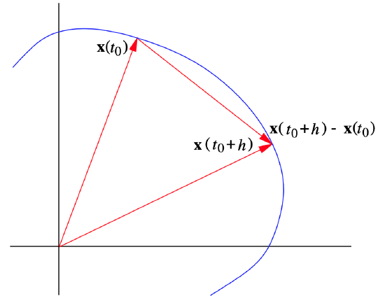
At a given time \(t_0\), the vector \(\mathbf{x}\left(t_{0}+h\right)-\mathbf{x}\left(t_{0}\right)\) represents the magnitude and direction of the change of position of the particle along \(C\) from time \(t_0\) to time \(t_0 + h\), as shown in Figure 2.3.1. Dividing by \(h\), we obtain a vector,

\[ \frac{\mathbf{x}\left(t_{0}+h\right)-\mathbf{x}\left(t_{0}\right)}{h}, \]

with the same direction, but with length approximating the average speed of the particle over the time interval from \(t_0\) to \(t_0 + h\). Assuming differentiability and taking the limit as \(h\) approaches 0, we have the following definition.

Figure \(\PageIndex{1}\): Motion along a curve \(C\)

Definition \(\PageIndex{1}\)

Suppose \(\mathbf{x}(t)\) is the position of a particle at time \(t\) moving along a curve \(C\) in \(\mathbb{R}^n\). We call

\[ \mathbf{v}(t)=\frac{d}{d t} \mathbf{x}(t) \]

the velocity of the particle at time \(t\) and we call

\[ s(t)=\|\mathbf{v}(t)\| \]

the speed of the particle at time \(t\). Moreover, we call

\[ \mathbf{a}(t)=\frac{d}{d t} \mathbf{v}(t) \]

the acceleration of the particle at time \(t\).

Example \(\PageIndex{1}\)

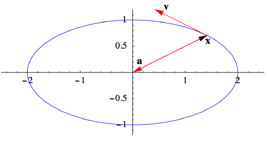
Consider a particle moving along an ellipse so that its position at any time \(t\)

\[\mathbf{x}=(2 \cos (t), \sin (t)). \nonumber \]

Then its velocity is

\[ \mathbf{v}=(-2 \sin (t), \cos (t)) , \nonumber \]

its speed is

\[ s=\sqrt{4 \sin ^{2}(t)+\cos ^{2}(t)}=\sqrt{3 \sin ^{2}(t)+1}, \nonumber \]

and its acceleration is

\[ \mathbf{a}=(-2 \cos (t),-\sin (t)). \nonumber \]

For example, at \(t=\frac{\pi}{4}\) we have

\[ \begin{gathered}
\left.\mathbf{x}\right|_{t=\frac{\pi}{4}}=\left(\sqrt{2}, \frac{1}{\sqrt{2}}\right), \\
\left.\mathbf{v}\right|_{t=\frac{\pi}{4}}=\left(-\sqrt{2}, \frac{1}{\sqrt{2}}\right), \\
\left.s\right|_{t=\frac{\pi}{4}}=\sqrt{\frac{5}{2}},
\end{gathered}\]

and

\[ \left.\mathbf{a}\right|_{t=\frac{\pi}{4}}=\left(-\sqrt{2},-\frac{1}{\sqrt{2}}\right) \text { . } \nonumber \]

See Figure 2.3.2. Notice that, in this example, \(\mathbf{a}=-\mathbf{x}\) for all values of \(t\).

Figure \(\PageIndex{2}\): Position, velocity, and acceleration vectors for motion on an ellipse

Curvature

Suppose \(\mathbf{x}\) is the position, \(\mathbf{v}\) is the velocity, \(s\) is the speed, and \(\mathbf{a}\) is the acceleration, at time \(t\), of a particle moving along a curve \(C\). Let \(T(t)\) be the unit tangent vector and \(N(t)\) be the principal unit normal vector at \(\mathbf{x}\). Now

\[ T(t)=\frac{\frac{d \mathbf{x}}{d t}}{\left\|\frac{d \mathbf{x}}{d t}\right\|}=\frac{\mathbf{v}}{\|\mathbf{v}\|}=\frac{\mathbf{v}}{s} , \]

so

\[\mathbf{v}=s\|T(t)\|. \]

Thus

\[ \mathbf{a}=\frac{d \mathbf{v}}{d t}=\frac{d}{d t} s T(t)=\frac{d s}{d t} T(t)+s D T(t) \]

Since

\[ N(t)=\frac{D T(t)}{\|D T(t)\|} ,\]

we have

\[ \mathbf{a}=\frac{d s}{d t} T(t)+s\|D T(t)\| N(t) . \label{2.3.10} \]

Note that (\(\ref{2.3.10}\)) expresses the acceleration of a particle as the sum of scalar multiples of the unit tangent vector and the principal unit normal vector. That is,

\[ \mathbf{a}=a_{T} T(t)+a_{N} N(t) ,\]

where

\[ a_{T}=\frac{d s}{d t} \]

and

\[ a_{N}=s\|D T(t)\|.\]

However, since \(T(t)\) and \(N(t)\) are orthogonal unit vectors, we also have

\[ \begin{align}
\mathbf{a} \cdot T(t) &=\left(a_{T} T(t)+a_{N} N(t)\right) \cdot T(t) \nonumber \\
&=a_{T}(T(t) \cdot T(t))+a_{N}(T(t) \cdot N(t)) \label{2.3.14}\\
&=a_{T} \nonumber
\end{align}\]

and

\[ \begin{align}
\mathbf{a} \cdot N(t) &=\left(a_{T} T(t)+a_{N} N(t)\right) \cdot N(t) c \nonumber \\
&=a_{T}(T(t) \cdot N(t))+a_{N}(N(t) \cdot N(t)) \label{2.3.15} \\
&=a_{N} . \nonumber
\end{align} \]

Hence \(a_T\) is the coordinate of \(\mathbf{a}\) in the direction of \(T(t)\) and \(a_N\) is the coordinate of \(\mathbf{a}\) in the direction of \(N(t)\). Thus (\(\ref{2.3.10}\)) writes the acceleration as a sum of its component in the direction of the unit tangent vector and its component in the direction of the principal unit normal vector. In particular, this shows that the acceleration lies in the plane determined by \(T(t)\) and \(N(t)\). Moreover, \(a_T\) is the rate of change of speed, while \(a_N\) is the product of the speed \(s\) and \(\|D T(t)\|\), the magnitude of the rate of change of the unit tangent vector. Since \(\|T(t)\|=1\) for all \(t\), \(\|D T(t)\|\) reflects only the rate at which the direction of \(T(t)\) is changing; in other words, \(\|D T(t)\|\) is a measurement of how fast the direction of the particle moving along the curve \(C\) is changing at time \(t\). If we divide this by the speed of the particle, we obtain a standard measurement of the rate of change of direction of \(C\) itself.

Definition \(\PageIndex{2}\)

Given a curve \(C\) with smooth parametrization \(\mathbf{x}=f(t)\), we call

\[ \kappa=\frac{\|D T(t)\|}{s(t)} \label{2.3.16}\]

the curvature of \(C\) at \(f(t)\).

Using (\(\ref{2.3.16}\)), we can rewrite (\(\ref{2.3.10}\)) as

\[ \mathbf{a}=\frac{d s}{d t} T(t)+s^{2} \kappa N(t) . \label{2.3.17} \]

Hence the coordinate of acceleration in the direction of the tangent vector is the rate of change of the speed and the coordinate of acceleration in the direction of the principal normal vector is the square of the speed times the curvature. Thus the greater the speed or the tighter the curve, the larger the size of the normal component of acceleration; the greater the rate at which speed is increasing, the greater the tangential component of acceleration. This is why drivers are advised to slow down while approaching a curve, and then to accelerate while driving through the curve.

Example \(\PageIndex{2}\)

Suppose a particle moves along a line in \(\mathbb{R}^n\) so that its position at any time \(t\) is given by

\[ \mathbf{x}=t \mathbf{w}+\mathbf{p} , \nonumber \]

where \(\mathbf{w} \neq 0\) and \(\mathbf{p}\) are vectors in \(\mathbb{R}^n\). Then the particle has velocity

\[ \mathbf{v}=\frac{d \mathbf{x}}{d t}=\mathbf{w} \nonumber \]

and speed \(\boldsymbol{s}=\|\mathbf{w}\|\), so the unit tangent vector is

\[ T(t)=\frac{\mathbf{v}}{s}=\frac{\mathbf{w}}{\|\mathbf{w}\|} . \nonumber \]

Hence \(T(t)\) is a constant vector, so \(D T(t)=\mathbf{0}\) and

\[ \kappa=\frac{\|D T(t)\|}{s}=0 \nonumber \]

for all \(t\). In other words, a line has zero curvature, as we should expect since the tangent vector never changes direction.

Example \(\PageIndex{3}\)

Consider a particle moving along a circle \(C\) in \(\mathbb{R}^2\) of radius \(r>0\) and center \((a,b)\), with its position at time given by

\[ \mathbf{x}=(r \cos (t)+a, r \sin (t)+b) . \nonumber \]

Then its velocity, speed, and acceleration are

\begin{gathered}
\mathbf{v}=(-r \sin (t), r \cos (t)), \\
s=\sqrt{\left.r^{2} \sin ^{(} t\right)+r^{2} \cos ^{2}(t)}=r
\end{gathered}

and

\[\mathbf{a}=(-r \cos (t),-r \sin (t)) , \nonumber \]

respectively. Hence the unit tangent vector is

\[ T(t)=\frac{\mathbf{v}}{s}=(-\sin (t), \cos (t)) . \nonumber \]

Thus

\[ D T(t)=(-\cos (t),-\sin (t)) \nonumber \]

and

\[ \|D T(t)\|=\sqrt{\cos ^{2}(t)+\sin ^{2}(t)}=1 .\nonumber \]

Hence the curvature of \(C\) is, for all \(t\),

\[ \kappa=\frac{\|D T(t)\|}{s}=\frac{1}{r} .\nonumber \]

Thus a circle has constant curvature, namely, the reciprocal of the radius of the circle. In particular, the larger the radius of a circle, the smaller the curvature. Also, note that

\[ \frac{d s}{d t}=\frac{d}{d t} r=0 , \nonumber \]

so, from (\(\ref{2.3.10}\)), we have

\[ \mathbf{a}=r N(t) , \nonumber \]

which we can verify directly. That is, the acceleration has a normal component, but no tangential component.

Example \(\PageIndex{4}\)

Now consider a particle moving along an ellipse \(E\) so that its position at any time \(t\) is

\[ \mathbf{x}=(2 \cos (t), \sin (t)) .\nonumber \]

Then, as we saw above, the velocity and speed of the particle are

\[ \mathbf{v}=(-2 \sin (t), \cos (t)) \nonumber \]

and

\[s=\sqrt{3 \sin ^{2}(t)+1} ,\nonumber \]

respectively. For purposes of differentiation, it will be helpful to rewrite \(s\) as

\[ s=\sqrt{\frac{3}{2}(1-\cos (2 t))+1}=\sqrt{\frac{5-3 \cos (2 t)}{2}} . \nonumber \]

Then the unit tangent vector is

\[ T(t)=\sqrt{\frac{2}{5-3 \cos (2 t)}}(-2 \sin (t), \cos (t)) . \nonumber \]

Thus

\[ D T(t)=\sqrt{\frac{2}{5-3 \cos (2 t)}}(-2 \cos (t),-\sin (t))-\frac{3 \sqrt{2} \sin (2 t)}{(5-3 \cos (2 t))^{\frac{3}{2}}}(-2 \sin (t), \cos (t)) . \nonumber \]

So, for example, at \(t=\frac{\pi}{4}\), we have

\[ \begin{gathered}
\left.\mathbf{x}\right|_{t=\frac{\pi}{4}}=\left(\sqrt{2}, \frac{1}{\sqrt{2}}\right), \\
\left.\mathbf{v}\right|_{t=\frac{\pi}{4}}=\left(-\sqrt{2}, \frac{1}{\sqrt{2}}\right), \\
\left.s\right|_{t=\frac{\pi}{4}}=\sqrt{\frac{5}{2}} ,
\end{gathered} \]

\[ \begin{aligned}
T\left(\frac{\pi}{4}\right) &=\frac{1}{\sqrt{5}}(-2,1) , \\
D T\left(\frac{\pi}{4}\right) &=-\frac{1}{5 \sqrt{5}}(4,8) ,
\end{aligned} \]

and

\[ \left\|D T\left(\frac{\pi}{4}\right)\right\|=\frac{1}{5 \sqrt{5}} \sqrt{16+64}=\frac{4}{5} . \nonumber \]

Hence the curvature of \(E\) at \(\left(\sqrt{2}, \frac{1}{\sqrt{2}}\right)\) is

\[ \left.\kappa\right|_{t=\frac{\pi}{4}}=\frac{\frac{4}{5}}{\sqrt{\frac{5}{2}}}=\frac{4 \sqrt{2}}{5 \sqrt{5}}=0.05060 , \nonumber \]

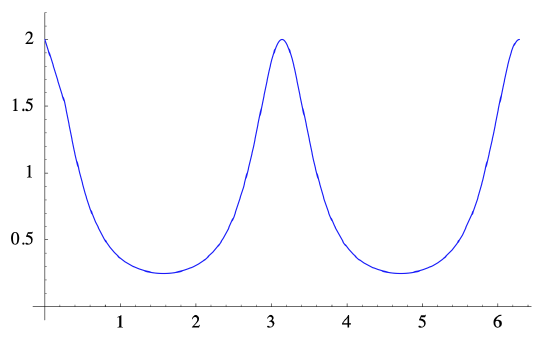
where the final numerical value has been rounded to four decimal places. Although the general expression for κ is complicated, it is easily computed and plotted using a computer algebra system, as shown in Figure 2.3.3. Comparing this with the plot of this ellipse in Figure 2.3.2, we can see why the curvature is greatest around (2,0) and (−2,0), corresponding to \(t=0\), \(t=\pi \), and \(t=2 \pi \), and smallest at (0,1) and (0,−1), corresponding to \(t=\frac{\pi}{2}\) and \(t=\frac{3 \pi}{2}\). Finally, as we saw above, the acceleration of the particle is

\[ \mathbf{a}=(-2 \cos (t),-\sin (t)), \nonumber \]

so

\[ \left.\mathbf{a}\right|_{t=\frac{\pi}{4}}=\left(-\sqrt{2},-\frac{1}{\sqrt{2}}\right) . \nonumber \]

Figure \(\PageIndex{3}\):: Curvature of an ellipse

Now if we write

\[ \left.\mathbf{a}\right|_{t=\frac{\pi}{4}}=a_{T} T(t)+a_{N} N(t), \nonumber \]

then we may either compute, using (\(\ref{2.3.17}\)),

\[ a_{T}=\left.\frac{d s}{d t}\right|_{t=\frac{\pi}{4}}=\frac{1}{\sqrt{2}}(5-3 \cos (2 t))^{-\frac{1}{2}}\left(\left.3 \sin (2 t)\right|_{t=\frac{\pi}{4}}=\frac{3}{\sqrt{10}}\right. \nonumber \]

and

\[ a_{N}=\left.\left.s^{2}\right|_{t=\frac{\pi}{4}} k\right|_{t=\frac{\pi}{4}}=\frac{5}{2} \frac{4 \sqrt{2}}{5 \sqrt{5}}=\frac{2 \sqrt{2}}{\sqrt{5}}=\frac{4}{\sqrt{10}}, \nonumber \]

or, using (\(\ref{2.3.14}\)) and (\(\ref{2.3.15}\)),

\[ a_{T}=\left.\mathbf{a}\right|_{t=\frac{\pi}{4}} \cdot T\left(\frac{\pi}{4}\right)=\left(-\sqrt{2},-\frac{1}{\sqrt{2}}\right) \cdot \frac{1}{\sqrt{5}}(-2,1)=\frac{3}{\sqrt{10}} \nonumber \]

and

\[ a_{N}=\left.\mathbf{a}\right|_{t=\frac{\pi}{4}} \cdot N\left(\frac{\pi}{4}\right)=\left(-\sqrt{2},-\frac{1}{\sqrt{2}}\right) \cdot \frac{1}{4 \sqrt{5}}(-4,-8)=\frac{4}{\sqrt{10}}. \nonumber \]

Hence, in either case,

\[ \left.\mathbf{a}\right|_{t=\frac{\pi}{4}}=\frac{3}{\sqrt{10}} T\left(\frac{\pi}{4}\right)+\frac{4}{\sqrt{10}} N\left(\frac{\pi}{4}\right) . \nonumber \]

Arc length

Suppose a particle moves along a curve \(C\) in \(\mathbb{R}^n\) so that its position at time \(t\) is given by \(\mathbf{x}=f(t)\) and let \(D\) be the distance traveled by the particle from time \(t=a\) to \(t=b\). We will suppose that \(s(t)=\|\mathbf{v}(t)\|\) is continuous on \( [a,b] \). To approximate \(D\), we divide \( [a,b]\) into \(n\) subintervals, each of length

\[ \Delta t=\frac{b-a}{n}, \nonumber \]

and label the endpoints of the subintervals \(a=t_{0}, t_{1}, \ldots, t_{n}=b\). If \(\Delta t\) is small, then the distance the particle travels during the \(j\)th subinterval, \(j=1,2, \ldots, n\), should be, approximately, \(s \Delta t\), an approximation which improves as \( \Delta t\) decreases. Hence, for sufficiently small \(\Delta t\)(equivalently, sufficiently large \(n\)),

\[ \sum_{j=1}^{n} s\left(t_{j-1}\right) \Delta t \label{2.3.18} \]

will provide an approximation as close to \(D\) as desired. That is, we should define

\[ D=\lim _{n \rightarrow \infty} \sum_{j=1}^{n} s\left(t_{j-1}\right) \Delta t . \label{2.3.19} \]

But (\(\ref{2.3.18}\)) is a Riemann sum (in particular, a left-hand rule sum) which approximates the definite integral

\[ \int_{a}^{b} s(t) d t . \label{2.3.20} \]

Hence the limit in (\(\ref{2.3.19}\)) is the value of the definite integral (\(\ref{2.3.20}\)), and so we have the following definition.

Definition \(\PageIndex{3}\)

Suppose a particle moves along a curve \(C\) in \(\mathbb{R}^n\) so that its position at time \(t\) is given by \(\mathbf{x}=f(t)\). Suppose the velocity \(\mathbf{v}(t)\) is continuous on the interval \([a,b]\). Then we define the distance traveled by the particle from time \(t=a\) to time \(t=b\) to be

\[ \int_{a}^{b}\|\mathbf{v}(t)\| d t . \label{2.3.21} \]

Note that the distance traveled is the length of the curve \(C\) if the particle traverses \(C\) exactly once. In that case, we call (\(\ref{2.3.21}\)) the length of \(C\). In general, for any \(t\) such that the interval \([a,t]\) is in the domain of \(f\), we may calculate

\[ \sigma(t)=\int_{a}^{t}\|\mathbf{v}(u)\| d u , \]

which we call the arc length function for \(C\).

Example \(\PageIndex{5}\)

Consider the helix \(H\) parametrized by

\[ f(t)=(\cos (t), \sin (t), t) . \nonumber \]

If we let \(L\) denote the length of one complete loop of the helix, then a particle traveling along \(H\) according to \(\mathbf{x}=f(t)\) will traverse this distance as \(t\) goes from 0 to \(2\pi\). Since

\[ \mathbf{v}(t)=(-\sin (t), \cos (t), 1) , \nonumber \]

we have

\[ \|\mathbf{v}(t)\|=\sqrt{\sin ^{2}(t)+\cos ^{2}(t)+1}=\sqrt{2} .\nonumber \]

Hence

\[ L=\int_{0}^{2 \pi} \sqrt{2} d t=2 \sqrt{2} \pi . \nonumber \]

Example \(\PageIndex{6}\)

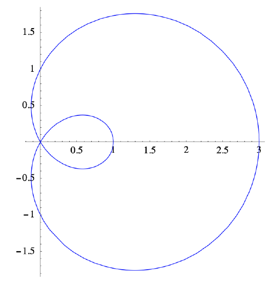
Suppose a particle moves along a curve \(C\) so that its position at time \(t\) is given by

\[ \mathbf{x}=((1+2 \cos (t)) \cos (t),(1+2 \cos (t)) \sin (t)) . \nonumber \]

Then \(C\) is the curve in Figure 2.3.4, which is called a limaçon. The particle will traverse this curve once as \(t\) goes from 0 to \(2\pi\). Now

\[ \mathbf{v}=\left(-(1+2 \cos (t)) \sin (t)-2 \sin (t) \cos (t),(1+2 \cos (t)) \cos (t)-2 \sin ^{2}(t)\right) , \nonumber \]

so

\begin{aligned}
\|\mathbf{v}\|^{2}=& \mathbf{v} \cdot \mathbf{v} \\
=&(1+2 \cos (t))^{2} \sin ^{2}(t)+4(1+2 \cos (t)) \sin ^{2}(t) \cos (t)+4 \sin ^{2}(t) \cos ^{2}(t), \\
& \quad+(1+2 \cos (t))^{2} \cos ^{2}(t)-4(1+2 \cos (t)) \sin ^{2}(t) \cos (t)+4 \sin ^{4}(t) \\
=&(1+2 \cos (t))^{2}\left(\sin ^{2}(t)+\cos ^{2}(t)\right)+4 \sin ^{2}(t) \cos ^{2}(t)+4 \sin ^{4}(t) \\
=&(1+2 \cos (t))^{2}+4 \sin ^{2}(t) \cos ^{2}(t)+4 \sin ^{4}(t)
\end{aligned}

Figure \(\PageIndex{4}\): A limaçon

Hence the length of \(C\) is

\[ \int_{0}^{2 \pi} \sqrt{(1+2 \cos (t))^{2}+4 \sin ^{2}(t) \cos ^{2}(t)+4 \sin ^{4}(t)} d t=13.3649 , \nonumber \]

where the integration was performed with a computer and the final result rounded to four decimal places. Note that integrating from 0 to \(4\pi\) would find the distance the particle travels in going around \(C\) twice, namely,

\[ \int_{0}^{4 \pi} \sqrt{(1+2 \cos (t))^{2}+4 \sin ^{2}(t) \cos ^{2}(t)+4 \sin ^{4}(t)} d t=26.7298 . \nonumber \]