6.1: An Introduction to Functions

The functions we studied in calculus are real functions, which are defined over a set of real numbers, and the results they produce are also real. In this chapter, we shall study their generalization over other sets. The definition could be difficult to grasp at the beginning, so we would start with a brief introduction.

Most students view real functions as computational devices. However, in the generalization, functions are not restricted to computation only. A better way to look at functions is their input-output relationship. Let \(f\) denote a function. Given an element (which need not be a number), we call the result from \(f\) the image of \(x\) under \(f\), and write \(f(x)\), which is read as “\(f\) of \(x\).”

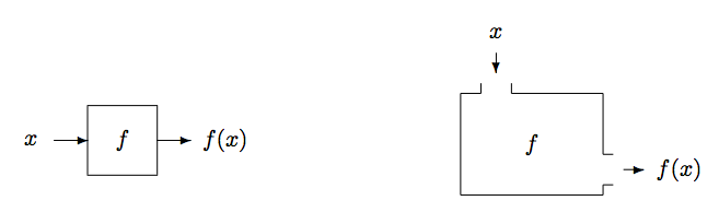
Imagine \(f\) as a machine. It takes the input value \(x\), and returns \(f(x)\) as the output value. This input-output relationship is depicted in Figure \(\PageIndex{1}\) in two different ways.

Figure \(\PageIndex{1}\): Two pictorial views of a function as a machine.

The question is: how could we obtain \(f(x)\)? A function need not involve any computation. Consequently, we cannot speak of “computing” the value of \(f(x)\). Instead, we talk about what is the rule we follow to obtain \(f(x)\). This rule can be described in many forms. We can, of course, use a computational rule. But a table, an algorithm, or even a verbal description also work as well.

When we say a real function is defined over the real numbers, we mean the input values must be real numbers. The output values are also real numbers. In general, the input and output values need not be of the same type. The nearest integer function, denoted \([x]\), rounds the real number \(x\) to the nearest integer. Here, the images (the output values) are integers. Consequently, we need to distinguish the set of input values from the set of possible output values. We call them the domain and the codomain, respectively, of the function.

Example \(\PageIndex{1}\label{eg:fcintro-1}\)

When a professor reports the final letter grades for the students in her class, we can regard this as a function \(g\). The domain is the set of students in her class, and the codomain could be the set of letter grades \(\{A, B, C, D, F\}\).

We said the codomain is the set of possible output values, because not every element in the codomain needs to appear as the image of some element from the domain. If no student fails the professor’s class in Example 6.1.1, no one will receive the final grade F. The collection of the images (the final letter grades) form a subset of the codomain. We call this subset the range of the function \(g\). The range of a function can be a proper subset of the codomain. Hence, the codomain of a function is different from the set of its images. If the range of a function does equal to the codomain, we say that the function is onto.

Example \(\PageIndex{2}\label{eg:fcintro-2}\)

For the nearest integer function \(h(x)=[x]\), the domain is \(\mathbb{R}\). The codomain is \(\mathbb{Z}\), and the range is also \(\mathbb{Z}\). Hence, the nearest integer function is onto.

Example \(\PageIndex{3}\label{eg:fcintro-3}\)

Let \(x\) be a real number. The greatest integer function \(\lfloor x\rfloor\) returns the greatest integer less than or equal to \(x\). For example, \[\big\lfloor \sqrt{50}\,\big\rfloor = 7, \qquad \lfloor -6.34 \rfloor = -7, \qquad\mbox{and}\qquad \lfloor 15 \rfloor = 15. \nonumber\] Therefore, \(\lfloor x\rfloor\) returns \(x\) if it is an integer, otherwise, it rounds \(x\) down to the next closest integer. Hence, it is also called the floor function of \(x\). It is clear that its domain is \(\mathbb{R}\), and the codomain and range are both \(\mathbb{Z}\).

hands-on exercise \(\PageIndex{1}\label{he:fcintro-1}\)

Let \(x\) be a real number. The least integer function \(\lceil x\rceil\) returns the least integer greater than or equal to \(x\). For example, \[\big\lceil \sqrt{50}\,\big\rceil = 8, \qquad \lceil -6.34 \rceil = -6, \qquad\mbox{and}\qquad \lceil 15 \rceil = 15. \nonumber\] Thus, \(\lceil x\rceil\) returns \(x\) if it is an integer, otherwise, it rounds \(x\) up to the next closest integer. Hence, it is also called the ceiling function of \(x\). What is its domain and codomain?

We impose two restrictions on the input-output relationships that we call functions. For any fixed input value \(x\), the output from a function must be the same every time we use the function. As a machine, it spits out the same answer every time we feed the same value \(x\) to it. As a calculator, it displays the same answer on its screen every time we enter the same value \(x\), and push the button for the function. We call the output value the image of \(x\), and write \(f(x)\). The first important requirement for a function \(f\) to be well-defined is: the image \(f(x)\) is unique for any fixed \(x\)-value.

A good machine must perform properly. In terms of a function \(f\), we must be able to obtain \(f(x)\) for any value \(x\) (and, of course, produce only one result for each \(x\)). This is perhaps a little bit too demanding. A remedy is to restrict our attention to those \(x\)’s over which \(f\) would work. The set of legitimate input values is precisely what we call the domain of the function. Consequently, the second requirement says: for every element \(x\) from the domain, the output value \(f(x)\) should be well-defined. This is the mathematical way of saying that the value \(f(x)\) can be obtained.

Example \(\PageIndex{4}\label{eg:fcintro-4}\)

Compare this to a calculator. If you enter a negative number and press the \(\sqrt{\phantom{x}}\,\) button, an error message will appear. To be able to compute the square root of a number, the number must be nonnegative. The domain of a function is the set of acceptable input values for which meaningful results can be found. For the square root function, the domain is \(\mathbb{R}^+\cup\{0\}\), which is the set of nonnegative real numbers.

hands-on exercise \(\PageIndex{2}\label{he:fcintro-2}\)

For the square root function, we may regard its codomain as \(\mathbb{R}\). What is its range? Is the function onto?

hands-on exercise \(\PageIndex{3}\label{he:fcintro-3}\)

For the square root function, can we say its domain is \(\mathbb{R}^+\cup0\)? Explain.

The two conditions for a function to be well-defined are often combined and written as if it were only one condition:

A function \(f\) is well-defined if every element \(x\) from the domain has a unique image in the codomain.

When you examine this definition closer, you will find the two separate requirements:

• every element in the domain has an image under \(f\), and
• the image is unique.

In the next section, we shall present the complete formal definition.

Summary and Review

• A function is a rule that assigns to every element in the domain a unique image in the codomain.

exercise \(\PageIndex{1}\label{ex:fcintro-1}\)

Complete the following table:

\[ \begin{array}{|c||c|c|c|c|c|c|} \hline x & 5.7 & \pi & e & -7.2 & -0.8 & 9 \\ \hline \lfloor x \rfloor & \qquad\qquad & \qquad\qquad & \qquad\qquad & \qquad\qquad & \qquad\qquad & \qquad\qquad \\ \lceil x \rceil &&&&&& \\ {[x]} &&&&&& \\ \hline \end{array} \nonumber\]

exercise \(\PageIndex{2}\label{ex:fcintro-2}\)

What is the domain and the codomain of the cube root function? Is it onto?

exercise \(\PageIndex{3}\label{ex:fcintro-3}\)

For the square root function, how would you use the interval notation to describe the domain?

exercise \(\PageIndex{4}\label{ex:fcintro-4}\)

For the square root function, which set complement would you use to describe the domain?