4.5: Dirichlet and Lambert Series

We will take a quick look at some interesting series without worrying too much about their convergence, because we are ultimately interested in the analytic continuations that underlie these series. For that, it is sufficient that there is convergence in any open non-empty region of the complex plane.

Definition 4.18

Let \(f, g\), and \(F\) be arithmetic functions (see Definition 4.1). Define the Dirichlet convolution of \(f\) and \(g\), denoted by \(f \star g\), as

\[(f \ast g)(n) \equiv \sum_{ab=n} f(a)g(b) \nonumber\]

This convolution is a very handy tool. Similar to the usual convolution of sequences, one can think of it as a sort of multiplication. It pays off to first define a few standard number theoretic functions.

Definition 4.19

We use the following notation for certain standard sequences. The sequence \(\epsilon (n\) is \(1\) if \(n = 1\) and otherwise returns \(0\), \(\textbf{1} (n)\) always returns \(1\), and \(I(n)\) returns \(n (I(n) = n)\).

The function \(\epsilon\) acts as the identity of the convolution. Indeed, \((\epsilon \ast f)(n) = \sum_{ab=n} \epsilon(a) f(b) = f(n)\).

Note that \(I(n)\) is the identity as a function, but should not be confused with the identity of the convolution \((\epsilon)\). In other words, \(I(n) = n\) but \(I \ast f \ne f\).

We can now do some very cool things of which we can unfortunately give but a few examples. As a first example, we reformulate the Mo ̈bius inversion of Theorem 4.14 as follows:

\[F = \textbf{1} \ast f \Leftrightarrow f = \mu \ast F \nonumber\]

This leads to the next example. The first of the following equalities holds by Lemma 4.15, the second follows from Mobius inversion.

\[I = \textbf{1} \ast \varphi \Leftrightarrow \varphi = \mu \ast I \nonumber\]

And the best of these examples is gotten by substituting the identity \(\epsilon\) for \(F\) in equation (4.5):

\[\epsilon = \textbf{1} \ast f \Leftrightarrow f = \mu \ast \epsilon = \mu \nonumber\]

Thus \(\mu\) is the convolution inverse of the sequence \((1,1,1 \cdots)\). This immediately leads to an unexpected expression for \(1/ \zeta (s)\) of equation (4.8).

Definition 4.20

Let \(f(n)\) is an arithmetic function (or sequence). A Dirichlet series is a series of the form \(F(s) = \sum_{n=1} f(n) n^{-s}\). Similarly, a Lambert series is a series of the form \(F(x) = \sum_{n=1} f(n) \frac{x^n}{1-x^n}\)

The prime example of a Dirichlet series is – of course – the Riemann zeta function of Definition 2.19, \(\zeta(s) = \sum \textbf{1} (n) n^{-s}\).

Theorem 4.21

For the product of two Dirichlet series we have

\[(\sum_{n=1} f(n)n^{-s})(\sum_{n=1} g(n)n^{-s}) = \sum_{n=1}^{\infty} (f \ast g) (n) n^{-s} \nonumber\]

Proof

This follows easily from re-arranging the terms in the product:

\[\sum_{a,b \ge 1}^{\infty} \frac{f(a) g(b)}{(ab)^s} = \sum_{n=1}^{\infty}(\sum_{n=1}^{\infty} f(a)g(b)) n^{-s} \nonumber\]

We collected the terms with \(ab = n\).

Since \(\frac{\zeta (s)}{\zeta(s)} = 1\), equation (4.7) and the lemma immediately imply that

\[\frac{1}{\zeta (s)} =\sum_{n \ge 1} \frac{\mu(n)}{n^s} \nonumber\]

Recall from Chapter 2 that one of the chief concerns of number theory is the location of the non-real zeros of \(\zeta\). At stake is Conjecture 2.22 which states that all its non-real zeros are on the line \(Re s = 1/2\). The original definition of the zeta function is as a series that is absolutely convergent for \(Re s > 1\) only. Thus it is important to establish that the analytic continuation of \(\zeta\) is valid for \(Re s \le 1\). The next result serves as a first indication that \(\zeta (s)\) can indeed be continued for values \(Re s \le 1\).

Theorem 4.22

Let \(\zeta\) be the Riemann zeta function and \(\sigma_{k}\) as in Definition 4.4, then

\[\zeta (s-k) \zeta (s) =\sum_{n=1}^{\infty} \frac{\sigma_{k} (n)}{n^s} \nonumber\]

Proof

\[\zeta (s-k) \zeta (s) = \sum_{a \ge 1} a^{-s} \sum_{b \ge 1} b^{k} b^{-s} = \sum_{n \ge 1} n^{-s} \sum_{b|n} b^k \nonumber\]

Lemma 4.23

A Lambert series can re-summed as follows:

\[\sum_{n=1}^{\infty} f(n) \frac{x^n}{1-x^n} = \sum_{n=1}^{\infty} (\textbf{1} \ast f) (n) x^{n} \nonumber\]

Proof

First use that

\[\frac{x^b}{1-x^b} = \sum_{a=1}^{\infty} x^{ab} \nonumber\]

This gives that

\[\sum_{n=1}^{\infty} f(b) \frac{x^b}{1-x^b} = \sum_{b=1}^{\infty} \sum_{a=1}^{\infty} f(b) x^{ab} \nonumber\]

Now set \(n = ab\) and collect terms. Noting that (\textbf{1} \ast f) (b) = \sum_{b \nmid n} f(b)\) yields the result.

Corollary 4.24

The following equality holds

\[\sum_{n \ge 1} \varphi (n) \frac{x^n}{1-x^n} = \frac{x}{(1-x)^2} \nonumber\]

Proof

We have

\[\sum_{n \ge 1} \varphi (n) \frac{x^n}{1-x^n} = \sum_{n \ge 1} (\textbf{1} \ast \varphi) (n) x^n = \sum_{n \ge 1} I(n) x^n \nonumber\]

The first equality follows from Lemma 4.23 and the second from Lemma 4.15. The last sum can be computed as \(x \frac{d}{dx} (1-x)^{-1}\) which gives the desired expression.

The last result is of importance in the study of dynamical systems. In figure 8, the map \(f_{t}\) is constructed by truncating the map \(x \rightarrow 2x\) mod \(1\) for \(t \in [0, 1]\). Corollary 4.24 can be used to show that the set of \(t\) for which \(f_{t}\) does not have a periodic orbit has measure (“length”) zero [24, 25], even though that set is uncountable.

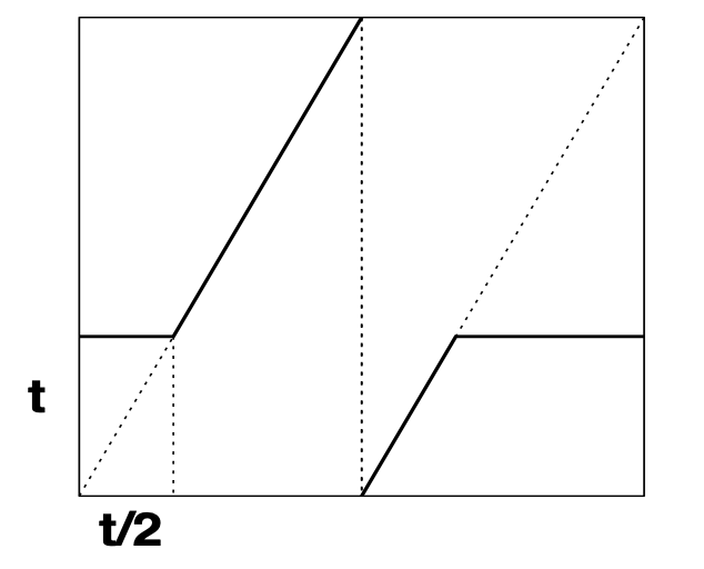
Figure 8. A one parameter family \(f_{t}\) of maps from the circle to itself. For every \(t \in [0, 1]\) the map \(f_{t}\) is constructed by truncating the map \(x \rightarrow 2x\) mod \(1\) as indicated in this figure.