6.2: Graphs of Relations on a Set

Last updated
Save as PDF

Page ID: 80522

$ \newcommand{\vecs}[1]{\overset { \scriptstyle \rightharpoonup} {\mathbf{#1}} } $

$ \newcommand{\vecd}[1]{\overset{-\!-\!\rightharpoonup}{\vphantom{a}\smash {#1}}} $

$ \newcommand{\id}{\mathrm{id}}$ $ \newcommand{\Span}{\mathrm{span}}$

( \newcommand{\kernel}{\mathrm{null}\,}\) $ \newcommand{\range}{\mathrm{range}\,}$

$ \newcommand{\RealPart}{\mathrm{Re}}$ $ \newcommand{\ImaginaryPart}{\mathrm{Im}}$

$ \newcommand{\Argument}{\mathrm{Arg}}$ $ \newcommand{\norm}[1]{\| #1 \|}$

$ \newcommand{\inner}[2]{\langle #1, #2 \rangle}$

$ \newcommand{\Span}{\mathrm{span}}$

$ \newcommand{\id}{\mathrm{id}}$

$ \newcommand{\Span}{\mathrm{span}}$

$ \newcommand{\kernel}{\mathrm{null}\,}$

$ \newcommand{\range}{\mathrm{range}\,}$

$ \newcommand{\RealPart}{\mathrm{Re}}$

$ \newcommand{\ImaginaryPart}{\mathrm{Im}}$

$ \newcommand{\Argument}{\mathrm{Arg}}$

$ \newcommand{\norm}[1]{\| #1 \|}$

$ \newcommand{\inner}[2]{\langle #1, #2 \rangle}$

$ \newcommand{\Span}{\mathrm{span}}$ $ \newcommand{\AA}{\unicode[.8,0]{x212B}}$

$ \newcommand{\vectorA}[1]{\vec{#1}} % arrow$

$ \newcommand{\vectorAt}[1]{\vec{\text{#1}}} % arrow$

$ \newcommand{\vectorB}[1]{\overset { \scriptstyle \rightharpoonup} {\mathbf{#1}} } $

$ \newcommand{\vectorC}[1]{\textbf{#1}} $

$ \newcommand{\vectorD}[1]{\overrightarrow{#1}} $

$ \newcommand{\vectorDt}[1]{\overrightarrow{\text{#1}}} $

$ \newcommand{\vectE}[1]{\overset{-\!-\!\rightharpoonup}{\vphantom{a}\smash{\mathbf {#1}}}} $

$ \newcommand{\vecs}[1]{\overset { \scriptstyle \rightharpoonup} {\mathbf{#1}} } $

$ \newcommand{\vecd}[1]{\overset{-\!-\!\rightharpoonup}{\vphantom{a}\smash {#1}}} $

$\newcommand{\avec}{\mathbf a}$ $\newcommand{\bvec}{\mathbf b}$ $\newcommand{\cvec}{\mathbf c}$ $\newcommand{\dvec}{\mathbf d}$ $\newcommand{\dtil}{\widetilde{\mathbf d}}$ $\newcommand{\evec}{\mathbf e}$ $\newcommand{\fvec}{\mathbf f}$ $\newcommand{\nvec}{\mathbf n}$ $\newcommand{\pvec}{\mathbf p}$ $\newcommand{\qvec}{\mathbf q}$ $\newcommand{\svec}{\mathbf s}$ $\newcommand{\tvec}{\mathbf t}$ $\newcommand{\uvec}{\mathbf u}$ $\newcommand{\vvec}{\mathbf v}$ $\newcommand{\wvec}{\mathbf w}$ $\newcommand{\xvec}{\mathbf x}$ $\newcommand{\yvec}{\mathbf y}$ $\newcommand{\zvec}{\mathbf z}$ $\newcommand{\rvec}{\mathbf r}$ $\newcommand{\mvec}{\mathbf m}$ $\newcommand{\zerovec}{\mathbf 0}$ $\newcommand{\onevec}{\mathbf 1}$ $\newcommand{\real}{\mathbb R}$ $\newcommand{\twovec}[2]{\left[\begin{array}{r}#1 \\ #2 \end{array}\right]}$ $\newcommand{\ctwovec}[2]{\left[\begin{array}{c}#1 \\ #2 \end{array}\right]}$ $\newcommand{\threevec}[3]{\left[\begin{array}{r}#1 \\ #2 \\ #3 \end{array}\right]}$ $\newcommand{\cthreevec}[3]{\left[\begin{array}{c}#1 \\ #2 \\ #3 \end{array}\right]}$ $\newcommand{\fourvec}[4]{\left[\begin{array}{r}#1 \\ #2 \\ #3 \\ #4 \end{array}\right]}$ $\newcommand{\cfourvec}[4]{\left[\begin{array}{c}#1 \\ #2 \\ #3 \\ #4 \end{array}\right]}$ $\newcommand{\fivevec}[5]{\left[\begin{array}{r}#1 \\ #2 \\ #3 \\ #4 \\ #5 \\ \end{array}\right]}$ $\newcommand{\cfivevec}[5]{\left[\begin{array}{c}#1 \\ #2 \\ #3 \\ #4 \\ #5 \\ \end{array}\right]}$ $\newcommand{\mattwo}[4]{\left[\begin{array}{rr}#1 \amp #2 \\ #3 \amp #4 \\ \end{array}\right]}$ $\newcommand{\laspan}[1]{\text{Span}\{#1\}}$ $\newcommand{\bcal}{\cal B}$ $\newcommand{\ccal}{\cal C}$ $\newcommand{\scal}{\cal S}$ $\newcommand{\wcal}{\cal W}$ $\newcommand{\ecal}{\cal E}$ $\newcommand{\coords}[2]{\left\{#1\right\}_{#2}}$ $\newcommand{\gray}[1]{\color{gray}{#1}}$ $\newcommand{\lgray}[1]{\color{lightgray}{#1}}$ $\newcommand{\rank}{\operatorname{rank}}$ $\newcommand{\row}{\text{Row}}$ $\newcommand{\col}{\text{Col}}$ $\renewcommand{\row}{\text{Row}}$ $\newcommand{\nul}{\text{Nul}}$ $\newcommand{\var}{\text{Var}}$ $\newcommand{\corr}{\text{corr}}$ $\newcommand{\len}[1]{\left|#1\right|}$ $\newcommand{\bbar}{\overline{\bvec}}$ $\newcommand{\bhat}{\widehat{\bvec}}$ $\newcommand{\bperp}{\bvec^\perp}$ $\newcommand{\xhat}{\widehat{\xvec}}$ $\newcommand{\vhat}{\widehat{\vvec}}$ $\newcommand{\uhat}{\widehat{\uvec}}$ $\newcommand{\what}{\widehat{\wvec}}$ $\newcommand{\Sighat}{\widehat{\Sigma}}$ $\newcommand{\lt}{<}$ $\newcommand{\gt}{>}$ $\newcommand{\amp}{&}$ $\definecolor{fillinmathshade}{gray}{0.9}$

In this section we introduce directed graphs as a way to visualize relations on a set.

Digraphs

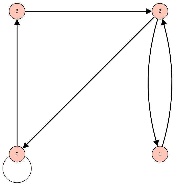
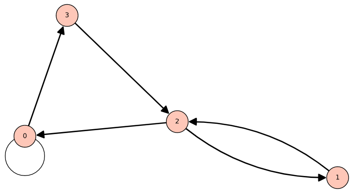
Let $A = \{0, 1,2,3\}\text{,}$ and let

\begin{equation*} r = \{(0, 0), (0, 3), (1, 2), (2, 1), (3, 2), (2, 0)\} \end{equation*}

In representing this relation as a graph, elements of $A$ are called the vertices of the graph. They are typically represented by labeled points or small circles. We connect vertex $a$ to vertex $b$ with an arrow, called an edge, going from vertex $a$ to vertex $b$ if and only if $a r b\text{.}$ This type of graph of a relation $r$ is called a directed graph or digraph. Figure $\PageIndex{1}$ is a digraph for $r\text{.}$ Notice that since 0 is related to itself, we draw a “self-loop” at 0.

The actual location of the vertices in a digraph is immaterial. The actual location of vertices we choose is called an embedding of a graph. The main idea is to place the vertices in such a way that the graph is easy to read. After drawing a rough-draft graph of a relation, we may decide to relocate the vertices so that the final result will be neater. Figure $\PageIndex{1}$ could also be presented as in Figure $\PageIndex{2}$.

A vertex of a graph is also called a node, point, or a junction. An edge of a graph is also referred to as an arc, a line, or a branch. Do not be concerned if two graphs of a given relation look different as long as the connections between vertices are the same in the two graphs.

Example $\PageIndex{1}$: Another Directed Graph

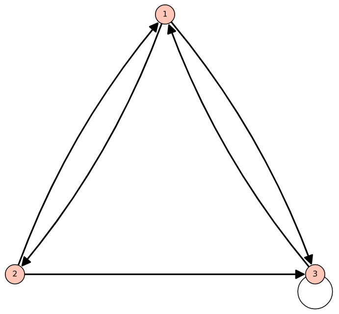
Consider the relation $s$ whose digraph is Figure $\PageIndex{3}$. What information does this give us? The graph tells us that $s$ is a relation on $A = \{1, 2, 3\}$ and that $s = \{(1, 2), (2, 1), (1, 3), (3, 1), (2, 3), (3, 3)\}\text{.}$

We will be building on the next example in the following section.

Example $\PageIndex{2}$: Ordering Subsets of a Two Element Universe

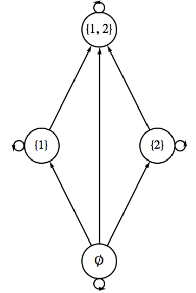
Let $B = \{1,2\}\text{,}$ and let $A = \mathcal{P}(B) = \{\emptyset, \{1\}, \{2\}, \{1,2\}\}\text{.}$ Then $\subseteq$ is a relation on $A$ whose digraph is Figure $\PageIndex{4}$.

$clipboard_e0427f4b66176bc81b0300cf2af0bc2af.png$ Figure $\PageIndex{4}$: Graph for set containment on subsets of $\{1,2\}$

We will see in the next section that since $\subseteq$ has certain structural properties that describe “partial orderings.” We will be able to draw a much simpler type graph than this one, but for now the graph above serves our purposes.

Exercises

Exercise $\PageIndex{1}$

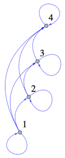
Let $A = \{1, 2, 3, 4\}\text{,}$ and let $r$ be the relation $\leq$ on $A\text{.}$ Draw a digraph for $r\text{.}$

Answer

$clipboard_ea09140ac71453cfb0834d7d54648dfe6.png$

Figure $\PageIndex{5}$: Digraph for $\leq$

$clipboard_e8ce2c5ec7978bdcc65babe2b61288e7f.png$

Figure $\PageIndex{6}$: Hasse diagram for $\leq$

Exercise $\PageIndex{2}$

Let $B = \{1,2, 3, 4, 6, 8, 12, 24\}\text{,}$ and let $s$ be the relation “divides” on $B\text{.}$ Draw a digraph for $s\text{.}$

Exercise $\PageIndex{3}$

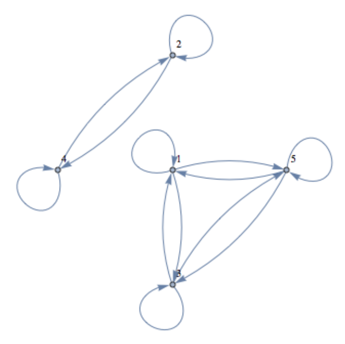
Let $A=\{1,2,3,4,5\}\text{.}$ Define $t$ on $A$ by $a t b$ if and only if $b - a$ is even. Draw a digraph for $t\text{.}$

Answer

See Figure $\PageIndex{7}$

$clipboard_eb94767f831aa7d090c52d93542450a20.png$

Figure $\PageIndex{7}$: Digraph of the relation $t$

Exercise $\PageIndex{4}$

Let $A$ be the set of strings of 0's and 1's of length 3 or less. This includes the empty string, $\lambda\text{,}$ which is the only string of length zero.

Define the relation of $d$ on $A$ by $x d y$ if $x$ is contained within $y\text{.}$ For example, $01 d 101\text{.}$ Draw a digraph for this relation.
Do the same for the relation $p$ defined by $x p y$ if $x$ is a prefix of $y\text{.}$ For example, $10 p 101\text{,}$ but $01 p 101$ is false.

Exercise $\PageIndex{5}$

Recall the relation in Exercise 6.1.5 of Section 6.1, $\rho$ defined on the power set, $\mathcal{P}(S)\text{,}$ of a set $S\text{.}$ The definition was $(A,B) \in \rho$ iff $A\cap B = \emptyset\text{.}$ Draw the digraph for $\rho$ where $S = \{a, b\}\text{.}$

Exercise $\PageIndex{6}$

Let $C= \{1,2, 3, 4, 6, 8, 12, 24\}$ and define $t$ on $C$ by $a t b$ if and only if $a$ and $b$ share a common divisor greater than 1. Draw a digraph for $t\text{.}$

Search

Text Color

Text Size

Margin Size

Font Type