19.6: Topological Sorting
- Page ID
- 93877
Sometimes we want to turn a partial order into a total order. What makes an order partial instead of total is the presence of pairs of incomparable elements. So to convert our partial order into a total order we just need to impose an order relation on those previously incomparable element pairs. However, for each pair of incomparable elements there is a choice to be made of which will become the smaller and which the larger in the new total order. And we cannot carry out these choices completely arbitrarily, because we risk contradicting the required properties of a partial order (see Example \(\PageIndex{1}\)).
The following definitions apply to a partial order \(\mathord{\preceq}\) on a set \(A\text{.}\)
Definition: Compatible Total Order
a total order \(\mathord{\le}\) on \(A\) such that if \(a_1 \preceq a_2\) then \(a_1 \le a_2\)
Definition: Topological Sorting
a process for determining a compatible total order
Example \(\PageIndex{1}\): A failed attempt at topological sorting.
The relation \(\mathord{\subseteq}\) on \(\mathscr{P}(\mathbb{N})\) is a partial order but not a total order. Consider what happens when we begin trying to build a total order on \(\mathscr{P}(\mathbb{N})\) out of \(\mathord{\subseteq}\) by choosing relations between previously incomparable elements arbitrarily.
- Elements \(\{1\},\{2,3\}\) are \(\mathord{\subseteq}\)-incomparable; choose \(\{2,3\} \le \{1\}\text{.}\)
- Elements \(\{1\},\{2\}\) are \(\mathord{\subseteq}\)-incomparable; choose \(\{1\} \le \{2\}\text{.}\)
- …
Now, \(\{2\} \subseteq \{2,3\}\) is already true, so to be compatible we must set \(\{2\} \leq \{2,3\}\) in the new total order. But now \(\{1\} \leq \{2\} \leq \{2,3\}\) would dictate \(\{1\} \leq \{2,3\}\) to satisfy the transitive property, but this contradicts our first arbitrary choice above.
If \(A\) is countable, whether finite or countably infinite, then specifying a total order on \(A\) amounts to writing the elements of \(A\) in an ordered list. (See Example 19.4.6 and Remark 19.4.7.) In that case, topological sorting amounts to creating such an ordered list so that if \(a \preceq b\) then \(a\) appears before \(b\) in the list.
If \(A\) is a finite partially ordered set with respect to \(\mathord{\preceq}\text{,}\) we can specify a compatible total order \(\mathord{\leq}\) on \(A\) by writing the elements of \(A\) in a list
\begin{equation*} a_0 \leq a_1 \leq \cdots \leq a_{n-1} \end{equation*}
as follows, where \(n = \vert A \vert\text{.}\)
- Initialize \(i = 0\) and \(A_0 = A\text{.}\)
- Choose a minimal element of \(A_i\text{;}\) let \(a_i\) represent the chosen element.
- Set \(A_{i+1} = A_i \setminus \{a_i\}\) (i.e. create a smaller partially ordered set by discarding \(a_i\)).
- Increment \(i\) by \(1\text{.}\) If \(i \lt n\) then go back to Step 2. Otherwise, if \(i = n\) then \(A_i\) should now be empty, so stop — the desired compatible order has now been specified.
In Step 2 of the algorithm, if \(A_i\) contains a minimum element, then you must choose that element, since in that case no other minimal element can exist (see the Fact 19.5.2).
Example \(\PageIndex{1}\)
Consider
\begin{equation*} A = \mathscr{P}(\{0,1,2\}) = \bigl\{ \emptyset, \{0\}, \{1\}, \{2\}, \{0,1\}, \{0,2\}, \{1,2\}, \{0,1,2\} \bigr\}\text{.} \end{equation*}
Apply Algorithm \(\PageIndex{1}\) to determine a total order \(\mathord{\leq}\) on \(A\) that is compatible with \(\mathord{\subseteq}\text{.}\)
Solution. 1 Algorithm solution
In \(A_0 = A\text{,}\) we must choose \(a_0 = \emptyset\text{,}\) since it is the minimum. Now remove \(a_0\) so that
\begin{equation*} A_1 = \bigl\{ \{0\}, \{1\}, \{2\}, \{0,1\}, \{0,2\}, \{1,2\}, \{0,1,2\} \bigr\}. \end{equation*}
Choose a minimal element from \(A_1\text{:}\) let \(a_1 = \{2\}\text{.}\) Now remove \(a_1\text{;}\) set
\begin{equation*} A_2 = \bigl\{ \{0\}, \{1\}, \{0,1\}, \{0,2\}, \{1,2\}, \{0,1,2\} \bigr\}. \end{equation*}
Choose a minimal element from \(A_2\text{:}\) let \(a_2 = \{0\}\text{.}\) Now remove \(a_2\text{;}\) set
\begin{equation*} A_3 = \bigl\{ \{1\}, \{0,1\}, \{0,2\}, \{1,2\}, \{0,1,2\} \bigr\}. \end{equation*}
Choose a minimal element from \(A_3\text{:}\) let \(a_3 = \{0,2\}\text{.}\) Now remove \(a_3\text{;}\) set
\begin{equation*} A_4 = \bigl\{ \{1\}, \{0,1\}, \{1,2\}, \{0,1,2\} \bigr\}. \end{equation*}
We must choose \(a_4 = \{1\}\text{,}\) since it is the minimum in \(A_4\text{.}\) Now remove \(a_4\text{;}\) set
\begin{equation*} A_5 = \bigl\{ \{0,1\}, \{1,2\}, \{0,1,2\} \bigr\}. \end{equation*}
Choose a minimal element from \(A_5\text{:}\) let \(a_5 = \{1,2\}\text{.}\) Now remove \(a_5\text{;}\) set \(A_6 = \bigl\{ \{0,1\}, \{0,1,2\} \bigr\}\text{.}\) We must choose \(a_6 = \{0,1\}\text{,}\) since it is the minimum in \(A_6\text{.}\) There is only one element left; set \(A_7 = \bigl\{ \{0,1,2\} \bigr\}\) and choose \(a_7 = \{0,1,2\}\text{.}\) So we have
\begin{equation*} \emptyset \leq \{2\} \leq \{0\} \leq \{0,2\} \leq \{1\} \leq \{1,2\} \leq \{0,1\} \leq \{0,1,2\}. \end{equation*}
Notice that the maximum element of \(A\) ended up at the “top” of the total order and the minimum element was forced to the “bottom.”
Solution. 2 Graphical solution
We can perform the algorithm of topological sorting graphically; at each step, choose a vertex that has no adjacent vertices below it in the graph, then cross that vertex and any adjacent edges out of the graph.
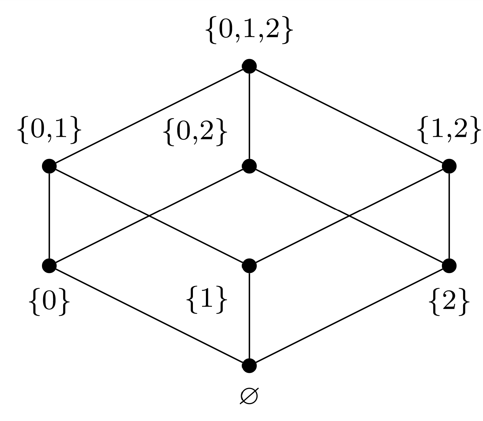
(a) Choose \(a_0 = \emptyset\text{.}\)
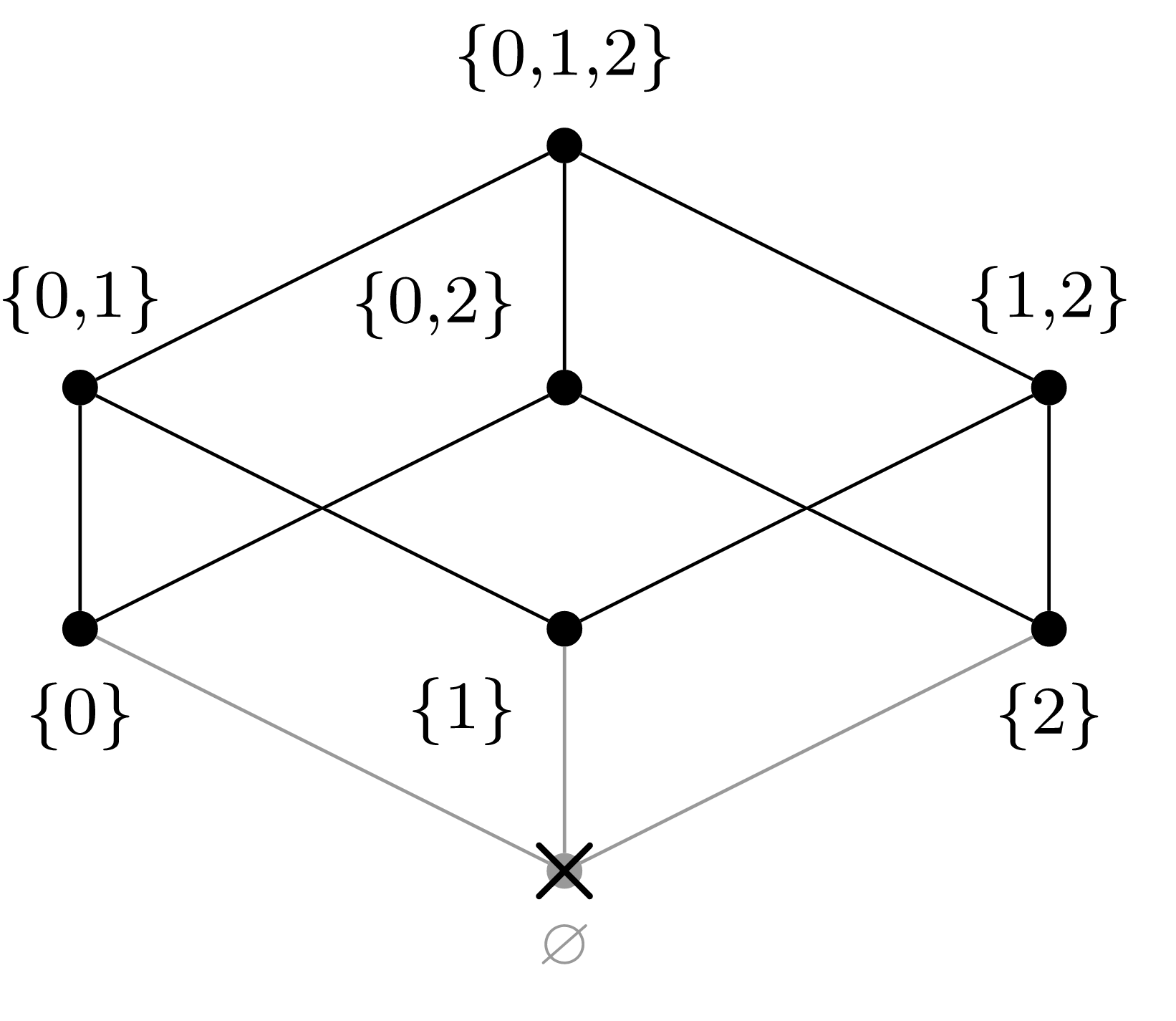
(b) Choose \(a_1 = \{2\}\text{.}\)
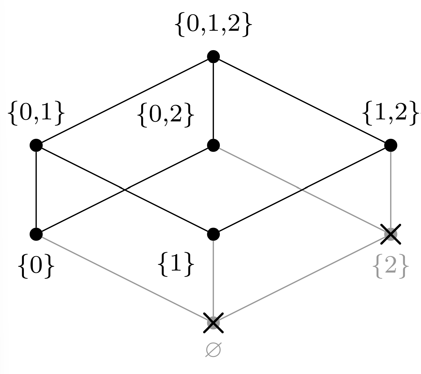
(c) Choose \(a_2 = \{0\}\text{.}\)
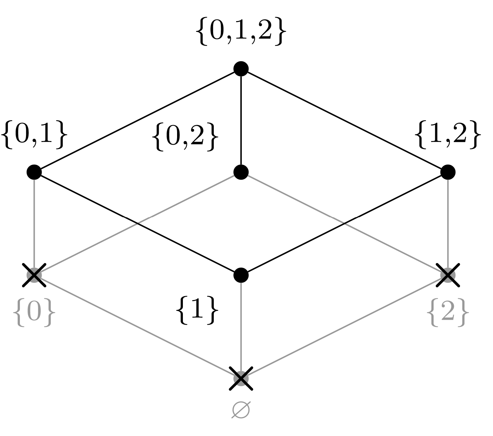
(d) Choose \(a_3 = \{0,2\}\text{.}\)
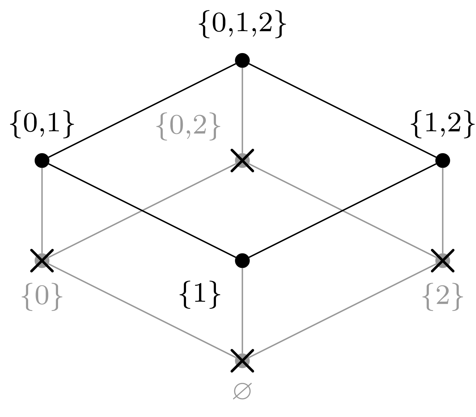
(e) Choose \(a_4 = \{1\}\text{.}\)
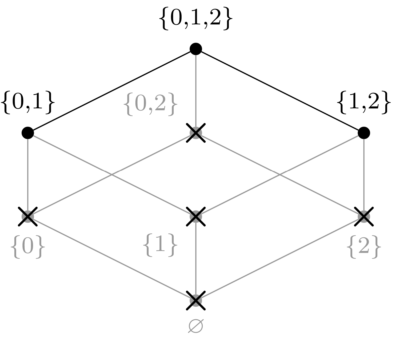
(f) Choose \(a_5 = \{1,2\}\text{.}\)
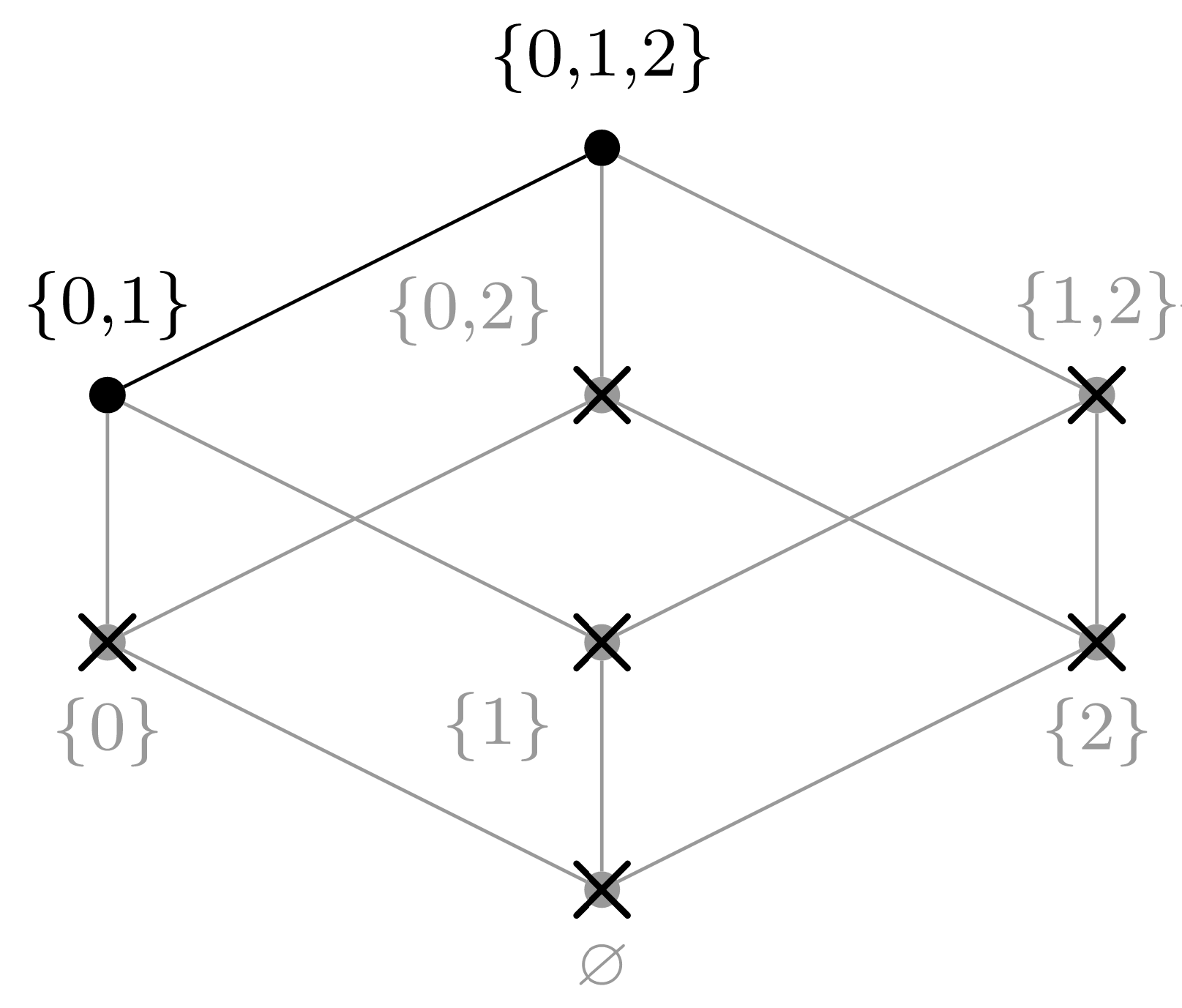
(g) Choose \(a_6 = \{0,1\}\text{.}\)
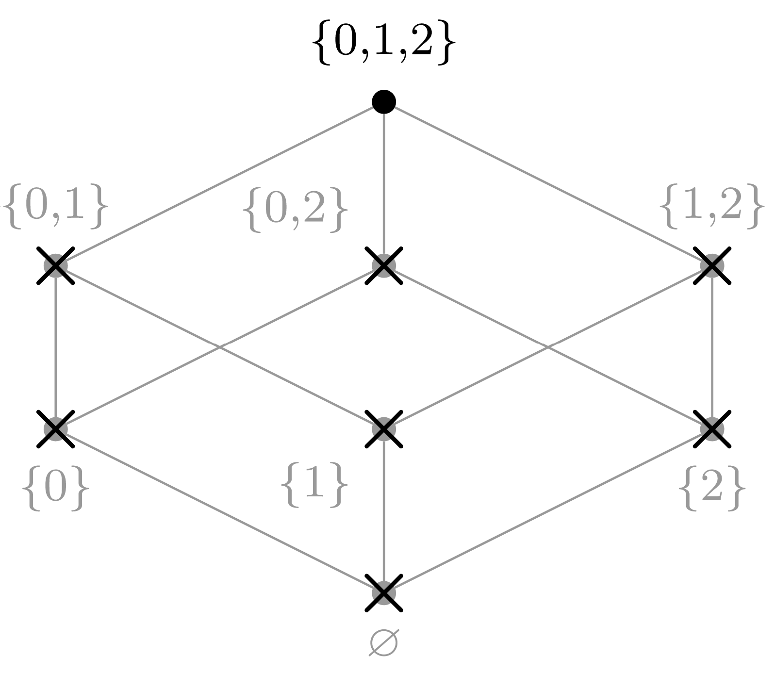
(h) Choose \(a_7 = \{0,1,2\}\text{.}\)
Figure \(\PageIndex{1}\): Paste Caption Here
Our end result is a list of our choices, in order:
Notice that the maximum element of \(A\) ended up at the “top” of the total order and the minimum element was forced to the “bottom”.
Compatible total orders are not unique: in the previous worked example, the order in which the elements of \(A\) were originally written represents another compatible total order:
\begin{equation*} \emptyset \leq \{0\} \leq \{1\} \leq \{2\} \leq \{0,1\} \leq \{0,2\} \leq \{1,2\} \leq \{0,1,2\} \text{.} \end{equation*}


