
2.3: Simple Harmonic Oscillators
- Page ID
- 91053

THE NEXT PHYSICAL PROBLEM OF INTEREST is that of simple harmonic motion. Such motion comes up in many places in physics and provides a generic first approximation to models of oscillatory motion. This is the beginning of a major thread running throughout this course. You have seen simple harmonic motion in your introductory physics class. We will review SHM (or SHO in some texts) by looking at springs, pendula (the plural of \(m\) pendulum), and simple circuits.
2.3.1: Mass-Spring Systems
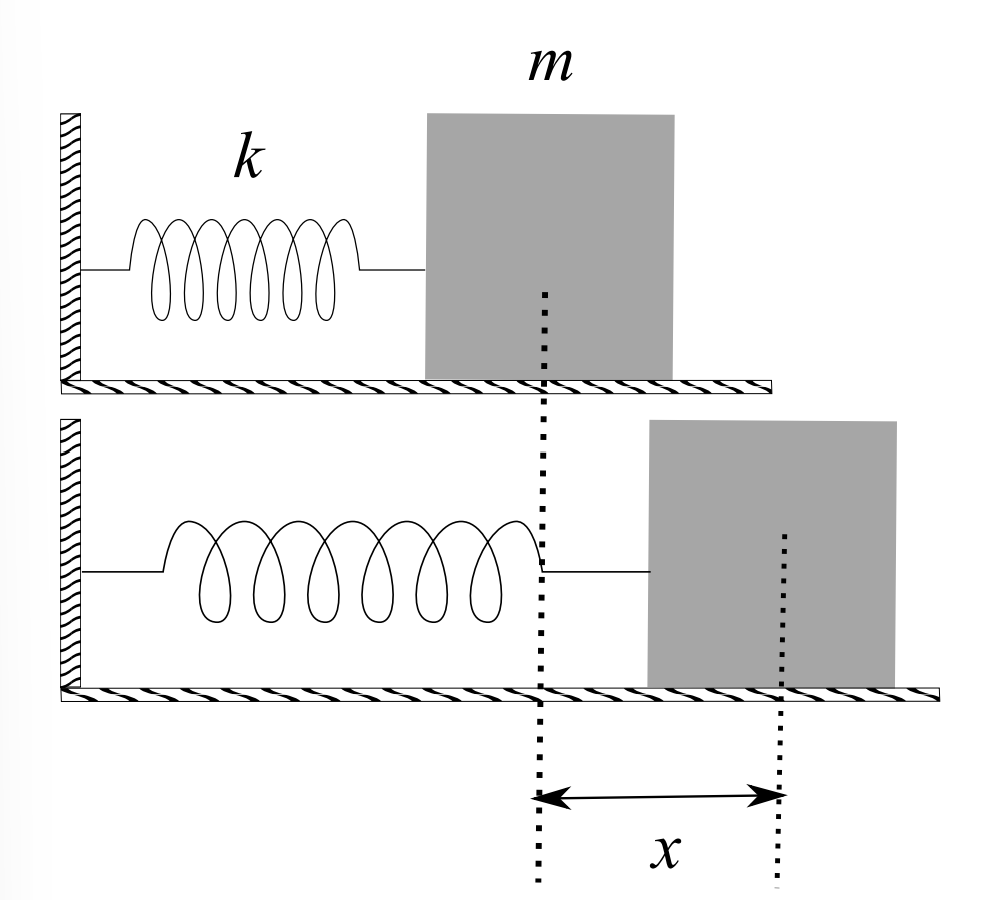
WE BEGIN WITH THE CASE of a single block on a spring as shown in Figure \(\PageIndex{1}\). The net force in this case is the restoring force of the spring given by Hooke’s Law,
\(F_{s}=-k x\)
where \(k>0\) is the spring constant. Here \(x\) is the elongation, or displacement of the spring from equilibrium. When the displacement is positive, the spring force is negative and when the displacement is negative the spring force is positive. We have depicted a horizontal system sitting on a frictionless surface. A similar model can be provided for vertically oriented springs. However, you need to account for gravity to determine the location of equilibrium. Otherwise, the oscillatory motion about equilibrium is modeled the same.
From Newton’s Second Law, \(F=m \ddot{x}\), we obtain the equation for the motion of the mass on the spring:
\[m \ddot{x}+k x=0 \label{2.19} \]
Dividing by the mass, this equation can be written in the form
\[\ddot{x}+\omega^{2} x=0 \nonumber \]
where
\(\omega=\sqrt{\dfrac{k}{m}}\)
This is the generic differential equation for simple harmonic motion.
We will later derive solutions of such equations in a methodical way. For now we note that two solutions of this equation are given by
\[ \begin{aligned} x(t) &=A \cos \omega t \\ x(t) &=A \sin \omega t \end{aligned} \label{2.21} \]
where \(\omega\) is the angular frequency, measured in rad/s, and \(A\) is called the amplitude of the oscillation.
The angular frequency is related to the frequency by
\(\omega=2 \pi f\)
where \(f\) is measured in cycles per second, or Hertz. Furthermore, this is related to the period of oscillation, the time it takes the mass to go through one cycle:
\(T=1 / f\)
2.3.2: The Simple Pendulum
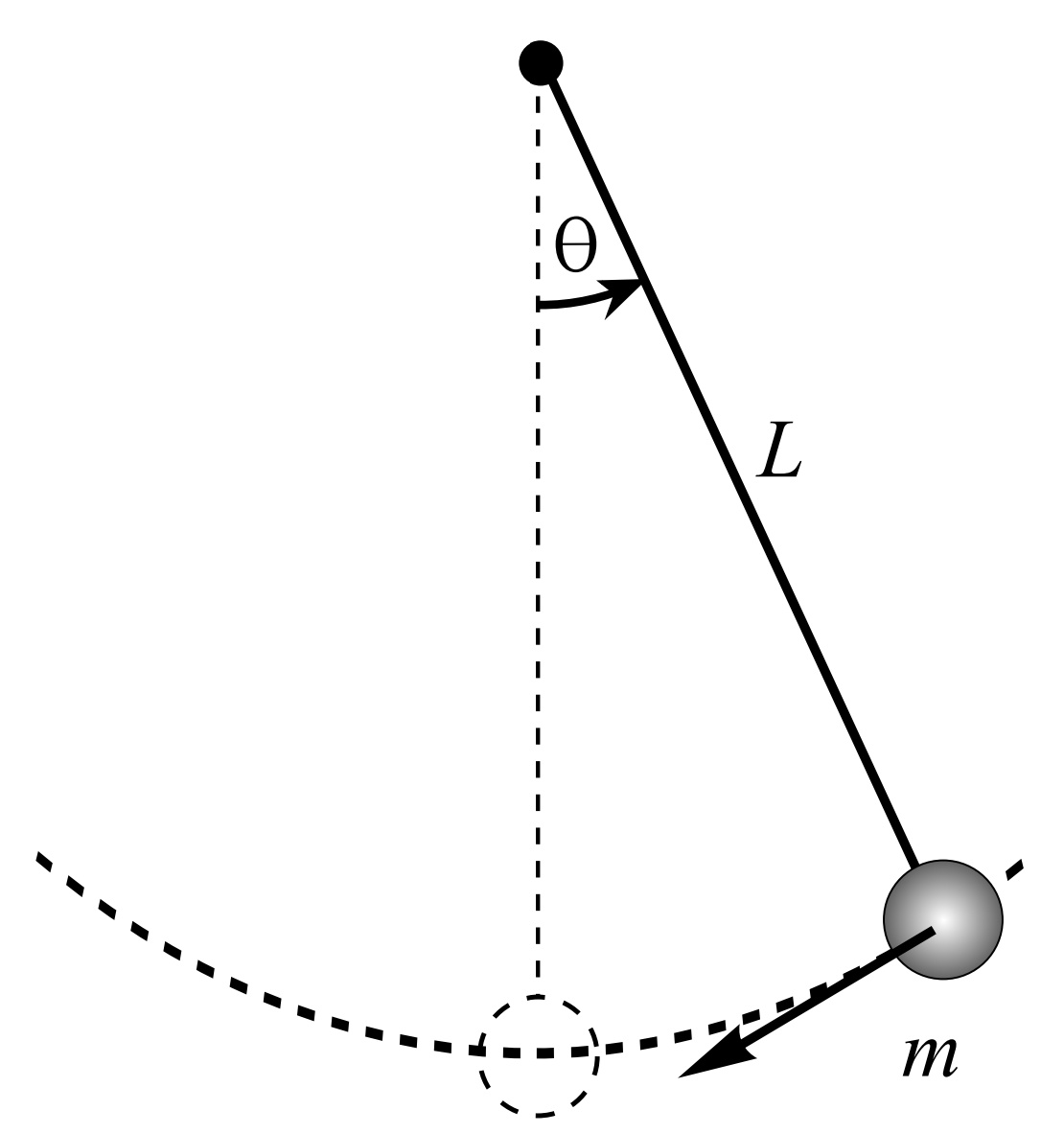
THE SIMPLE PENDULUM consists of a point mass \(m\) hanging on a string of length \(L\) from some support. [See Figure \(\PageIndex{2}\).] One pulls the mass back to some starting angle, \(\theta_{0}\), and releases it. The goal is to find the angular position as a function of time.
There are a couple of possible derivations. We could either use Newton’s Second Law of Motion, \(F=m a\), or its rotational analogue in terms of torque, \(\tau=I \alpha\). We will use the former only to limit the amount of physics background needed.
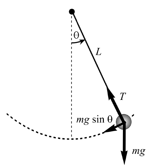
There are two forces acting on the point mass. The first is gravity. This points downward and has a magnitude of \(m g\), where \(g\) is the standard symbol for the acceleration due to gravity. The other force is the tension in the string. In Figure \(\PageIndex{3}\) these forces and their sum are shown. The magnitude of the sum is easily found as \(F=m g \sin \theta\) using the addition of these two vectors.
Now, Newton’s Second Law of Motion tells us that the net force is the mass times the acceleration. So, we can write
\(m \ddot{x} = -mg \sin \theta \)
Next, we need to relate \(x\) and \(\theta . x\) is the distance traveled, which is the length of the arc traced out by the point mass. The arclength is related to the angle, provided the angle is measure in radians. Namely, \(x=r \theta\) for \(r=L\). Thus, we can write
\(m L \ddot{\theta}=-m g \sin \theta .\)
Linear and nonlinear pendulum equation. Canceling the masses, this then gives us the nonlinear pendulum equation
\[L \ddot{\theta}+g \sin \theta=0 \nonumber \]
The equation for a compound pendulum takes a similar form. We start with the rotational form of Newton’s second law \(\tau=I \alpha\). Noting that the torque due to gravity acts at the center of mass position \(\ell\), the torque is given
\[\ddot{\theta}+\omega^{2} \theta=0 \nonumber \]
by \(\tau=-m g \ell \sin \theta\). Since \(\alpha=\ddot{\theta}\), we have \(I \ddot{\theta}=-m g \ell \sin \theta\). Then, for small angles \(\ddot{\theta}+\omega^{2} \theta=0\), where \(\omega=\dfrac{m g \ell}{I}\). For a simple pendulum, we let \(\ell=L\) and \(I=m L^{2}\), and obtain \(\omega=\sqrt{g / L} .\)
We note that this equation is of the same form as the mass-spring system. We define \(\omega=\sqrt{g / L}\) and obtain the equation for simple harmonic motion,
\(\ddot{\theta}+\omega^{2} \theta=0\)
There are several variations of Equation \(\PageIndex{4}\) which will be used in this text. The first one is the linear pendulum. This is obtained by making a small angle approximation. For small angles we know that \(\sin \theta \approx \theta .\) Under this approximation Equation \(\PageIndex{4}\) becomes
\[L \ddot{\theta}+g \theta=0 . \nonumber \]
2.3.3: LRC Circuits
ANOTHER TYPICAL PROBLEM OFTEN ENCOUNTERED in a first year physics class is that of an LRC series circuit. This circuit is pictured in Figure \(\PageIndex{4}\). The resistor is a circuit element satisfying Ohm’s Law. The capacitor is a device that stores electrical energy and an inductor, or coil, store magnetic energy.
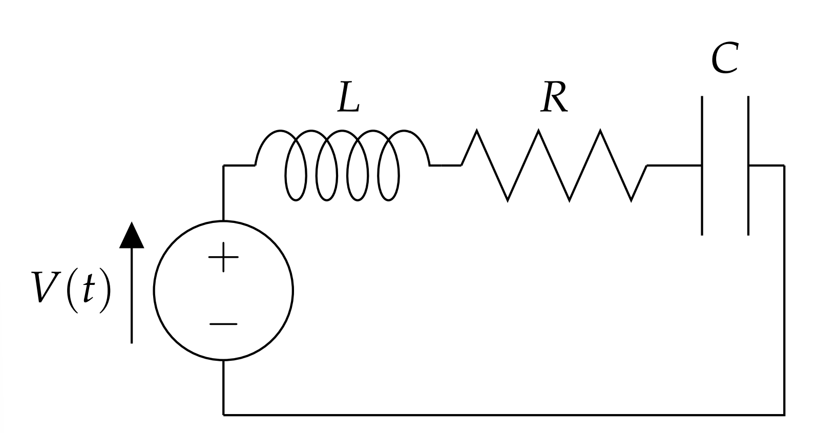
The physics for this problem stems from Kirchoff’s Rules for circuits. Namely, the sum of the drops in electric potential are set equal to the rises in electric potential. The potential drops across each circuit element are given by
- Resistor: \(V=I R .\)
- Capacitor: \(V=\dfrac{q}{C} .\)
- Inductor: \(V=L \dfrac{d I}{d t} .\)
Furthermore, we need to define the current as \(I=\dfrac{d q}{d t} .\) where \(q\) is the charge in the circuit. Adding these potential drops, we set them equal to the voltage supplied by the voltage source, \(V(t)\). Thus, we obtain
\(I R+\dfrac{q}{C}+L \dfrac{d I}{d t}=V(t)\)
Since both \(q\) and \(I\) are unknown, we can replace the current by its expression in terms of the charge to obtain
\(L \ddot{q}+R \dot{q}+\dfrac{1}{C} q=V(t)\)
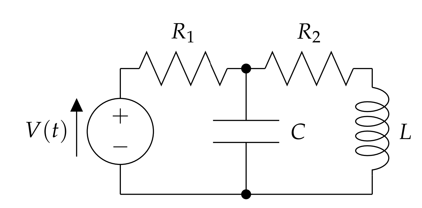
This is a second order equation for \(q(t)\). More complicated circuits are possible by looking at parallel connections, or other combinations, of resistors, capacitors and inductors. This will result in several equations for each loop in the circuit, leading to larger systems of differential equations. An example of another circuit setup is shown in Figure \(\PageIndex{5}\). This is not a problem that can be covered in the first year physics course. One can set up a system of second order equations and proceed to solve them. We will see how to solve such problems in the next chapter.
In the following we will look at special cases that arise for the series LRC circuit equation. These include RC circuits, solvable by first order methods and LC circuits, leading to oscillatory behavior.
2.3.4: RC Circuits
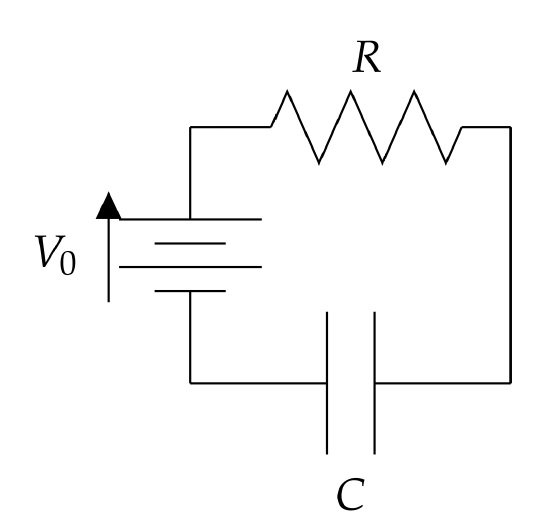
WE FIRST CONSIDER THE CASE OF an RC circuit in which there is no inductor. Also, we will consider what happens when one charges a capacitor with a DC battery \(\left(V(t)=V_{0}\right)\) and when one discharges a charged capacitor \((V(t)=0)\) as shown in Figures \(\PageIndex{6}\) and \(\PageIndex{9}\).
Charging a capacitor.
For charging a capacitor, we have the initial value problem
\[R \dfrac{d q}{d t}+\dfrac{q}{C}=V_{0}, \quad q(0)=0 \nonumber \]
This equation is an example of a linear first order equation for \(q(t) .\) However, we can also rewrite it and solve it as a separable equation, since \(V_{0}\) is a constant. We will do the former only as another example of finding the integrating factor.
We first write the equation in standard form:
\[\dfrac{d q}{d t}+\dfrac{q}{R C}=\dfrac{V_{0}}{R} \nonumber \]
The integrating factor is then
\(\mu(t)=e^{\int \dfrac{d t}{R C}}=e^{t / R C}\)
Thus,
\[\dfrac{d}{d t}\left(q e^{t / R C}\right)=\dfrac{V_{0}}{R} e^{t / R C} \nonumber \]
Integrating, we have
\[q e^{t / R C}=\dfrac{V_{0}}{R} \int e^{t / R C} d t=C V_{0} e^{t / R C}+K \nonumber \]
Note that we introduced the integration constant, \(K\). Now divide out the exponential to get the general solution:
\[q=C V_{0}+K e^{-t / R C} \nonumber \]
(If we had forgotten the \(K\), we would not have gotten a correct solution for the differential equation.)
Next, we use the initial condition to get the particular solution. Namely, setting \(t=0\), we have that
\(0=q(0)=C V_{0}+K\)
So, \(K=-C V_{0}\). Inserting this into the solution, we have
\[q(t)=C V_{0}\left(1-e^{-t / R C}\right) \nonumber \]
Now we can study the behavior of this solution. For large times the second term goes to zero. Thus, the capacitor charges up, asymptotically, to the final value of \(q_{0}=C V_{0} .\) This is what we expect, because the current is no longer flowing over \(R\) and this just gives the relation between the potential difference across the capacitor plates when a charge of \(q_{0}\) is established on the plates.
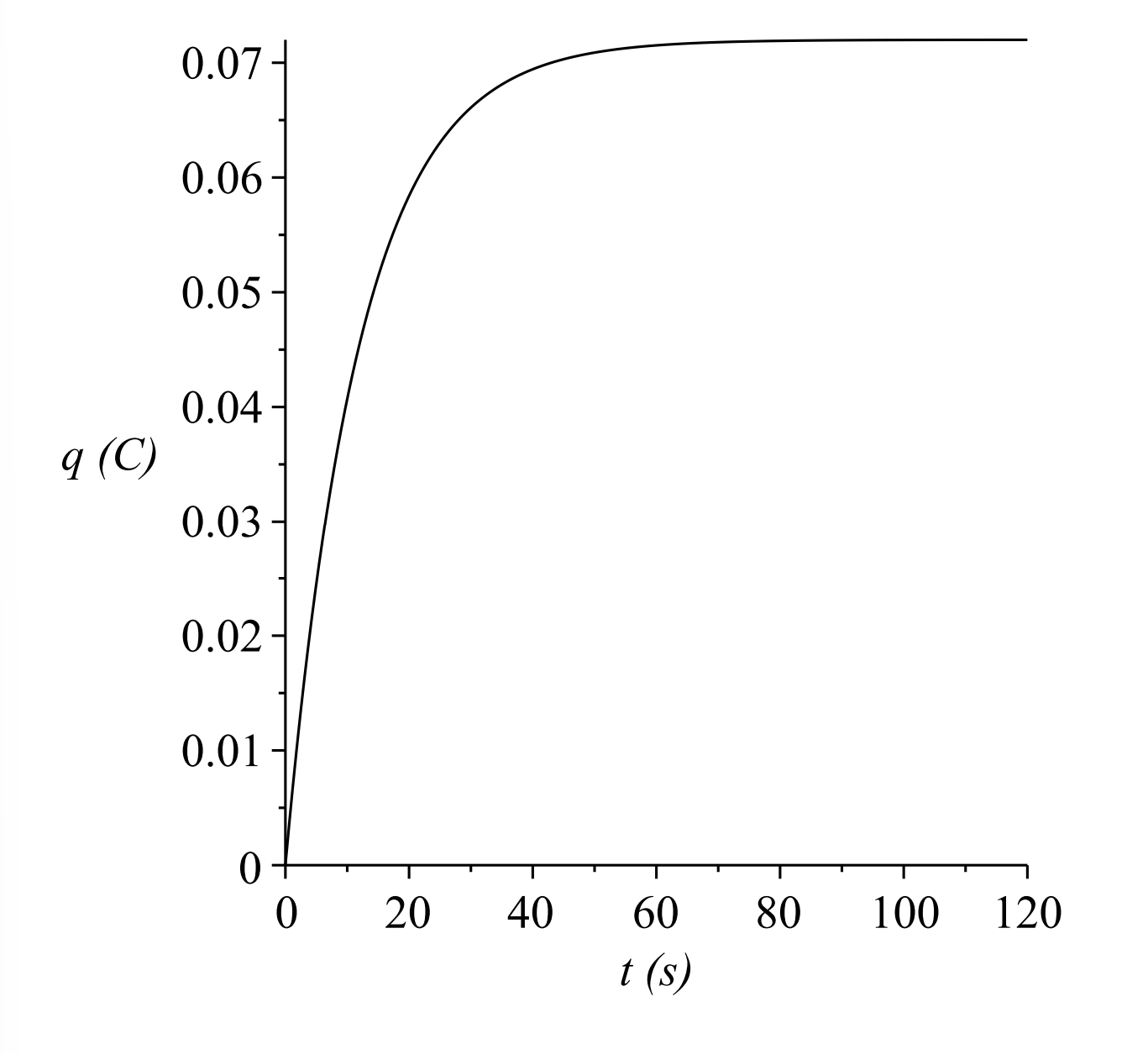
Let’s put in some values for the parameters. We let \(R = 2.00 k \omega \), \(C = 6.00\mathrm{mF}\), and \(V_{0}=12 \mathrm{~V} .\) A plot of the solution is given in Figure \(\PageIndex{7}\). We see that
the charge builds up to the value of \(C V_{0}=0.072 \mathrm{C}\). If we use a smaller
resistance, \(R=200 \Omega\), we see in Figure \(\PageIndex{8}\) that the capacitor charges to the
same value, but much faster.
Time constant, \(\tau=R C\).
The rate at which a capacitor charges, or discharges, is governed by the time constant, \(\tau=R C\). This is the constant factor in the exponential. The larger it is, the slower the exponential term decays. If we set \(t = \tau\), we find that
\(q(\tau)=C V_{0}\left(1-e^{-1}\right)=(1-0.3678794412 \ldots) q_{0} \approx 0.63 q_{0}\)
Thus, at time \(t=\tau\), the capacitor has almost charged to two thirds of its final value. For the first set of parameters, \(\tau=12 \mathrm{~s}\). For the second set, \(\tau=1.2 \mathrm{~s}\).
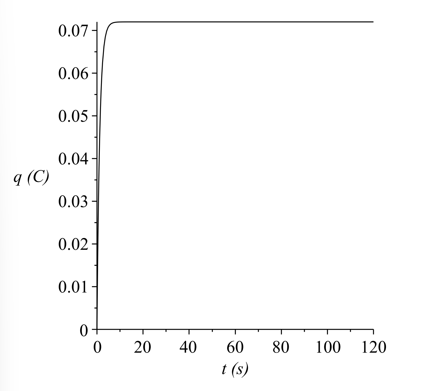 Figure \(\PageIndex{8}\): The charge as a function of time for a charging capacitor with \(R=200 \Omega\), \(C=6.00 \mathrm{mF}\), and \(V_{0}=12 \mathrm{~V}\)
Discharging a capacitor.
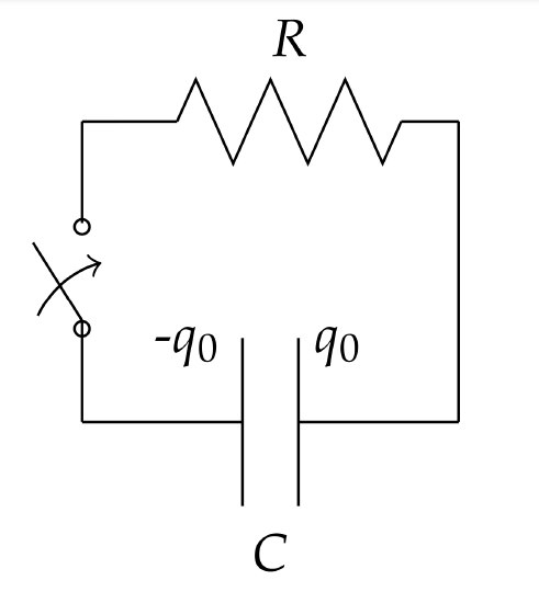
Now, let’s assume the capacitor is charged with charge \(\pm q_{0}\) on its plates. If we disconnect the battery and reconnect the wires to complete the circuit as shown in Figure \(\PageIndex{9}\), the charge will then move off the plates, discharging the capacitor. The relevant form of the initial value problem becomes
\[R \dfrac{d q}{d t}+\dfrac{q}{C}=0, \quad q(0)=q_{0} . \nonumber \]
This equation is simpler to solve. Rearranging, we have
\[\dfrac{d q}{d t}=-\dfrac{q}{R C} \nonumber \]
This is a simple exponential decay problem, which one can solve using separation of variables. However, by now you should know how to immediately write down the solution to such problems of the form \(y^{\prime}=k y\). The solution is
\(q(t)=q_{0} e^{-t / \tau}, \quad \tau=R C\)
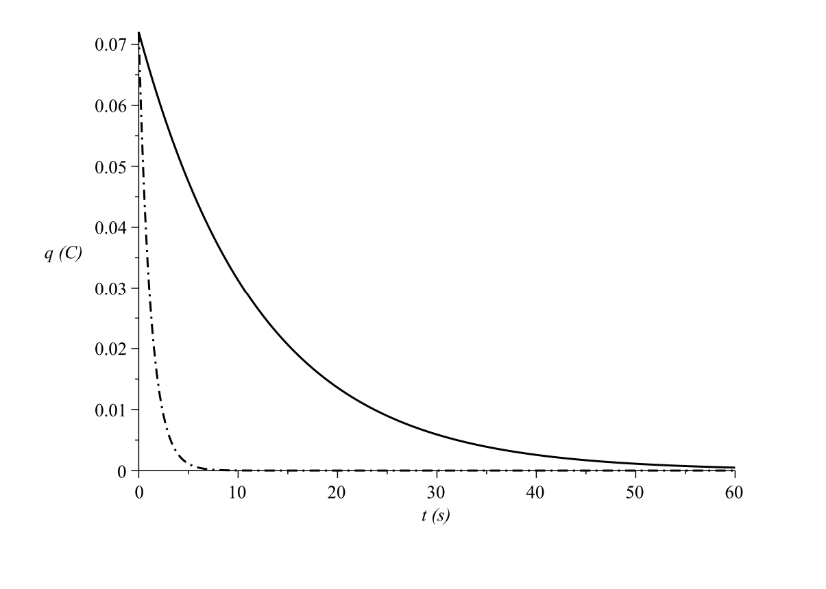
We see that the charge decays exponentially. In principle, the capacitor never fully discharges. That is why you are often instructed to place a shunt across a discharged capacitor to fully discharge it. In Figure \(\PageIndex{10} we show the discharging of the two previous RC circuits. Once again, \(\tau=R C\) determines the behavior. At \(t=\tau\) we have
\(q(\tau)=q_{0} e^{-1}=(0.3678794412 \ldots) q_{0} \approx 0.37 q_{0}\)
So, at this time the capacitor only has about a third of its original value.
2.3.5: LC Circuits
LC Oscillators.
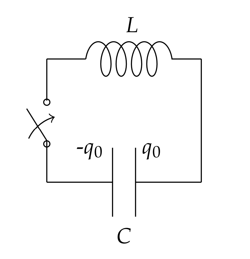
ANOTHER SIMPLE RESULT comes from studying \(L C\) circuits. We will now connect a charged capacitor to an inductor as shown in Figure \(\PageIndex{11}\). In this case, we consider the initial value problem
\[L \ddot{q}+\dfrac{1}{C} q=0, \quad q(0)=q_{0}, \dot{q}(0)=I(0)=0 \nonumber \]
Dividing out the inductance, we have
\[\ddot{q}+\dfrac{1}{L C} q=0 \nonumber \]
This equation is a second order, constant coefficient equation. It is of the same form as the ones for simple harmonic motion of a mass on a spring or the linear pendulum. So, we expect oscillatory behavior. The characteristic equation is
\(r^{2}+\dfrac{1}{L C}=0\)
The solutions are
\(r_{1,2}=\pm \dfrac{i}{\sqrt{L C}}\)
Thus, the solution of Equation \(\PageIndex{15}\) is of the form
\[ q(t)=c_{1} \cos (\omega t)+c_{2} \sin (\omega t), \quad \omega=(L C)^{-1 / 2} \nonumber \]
Inserting the initial conditions yields
\[q(t)=q_{0} \cos (\omega t) \nonumber \]
The oscillations that result are understandable. As the charge leaves the plates, the changing current induces a changing magnetic field in the inductor. The stored electrical energy in the capacitor changes to stored magnetic energy in the inductor. However, the process continues until the plates are charged with opposite polarity and then the process begins in reverse. The charged capacitor then discharges and the capacitor eventually returns to its original state and the whole system repeats this over and over.
The frequency of this simple harmonic motion is easily found. It is given by
\[f=\dfrac{\omega}{2 \pi}=\dfrac{1}{2 \pi} \dfrac{1}{\sqrt{L C}} \nonumber \]
This is called the tuning frequency because of its role in tuning circuits.
Find the resonant frequency for \(C=10 \mu \mathrm{F}\) and \(L=\) \(100 \mathrm{mH}\).
\(f=\dfrac{1}{2 \pi} \dfrac{1}{\sqrt{\left(10 \times 10^{-6}\right)\left(100 \times 10^{-3}\right)}}=160 \mathrm{~Hz}\)
Of course, this is an ideal situation. There is always resistance in the circuit, even if only a small amount from the wires. So, we really need to account for resistance, or even add a resistor. This leads to a slightly more complicated system in which damping will be present.
2.3.6: Damped Oscillations
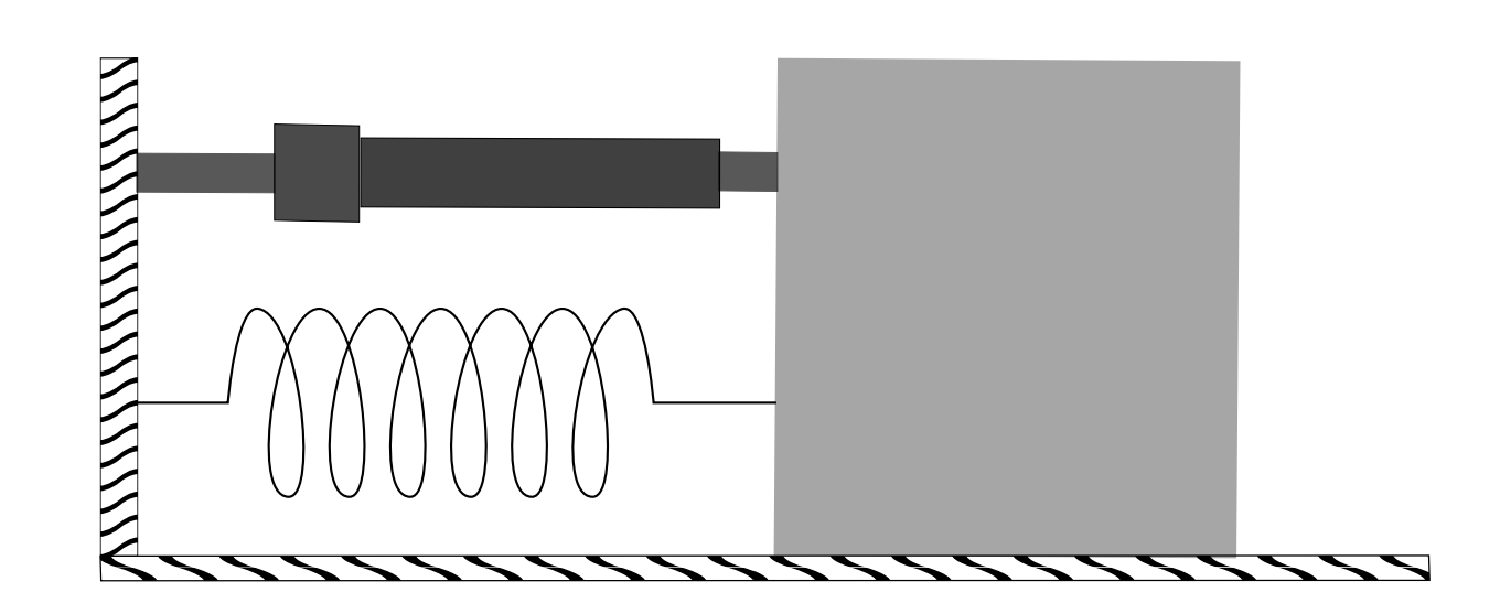
As WE HAVE INDICATED, simple harmonic motion is an ideal situation. In real systems we often have to contend with some energy loss in the system. This leads to the damping of the oscillations. A standard example is a spring-mass-damper system as shown in Figure \(2.12 \mathrm{~A}\) mass is attached to a spring and a damper is added which can absorb some of the energy of the oscillations. the damping is modeled with a term proportional to the velocity.
There are other models for oscillations in which energy loss could be in the spring, in the way a pendulum is attached to its support, or in the resistance to the flow of current in an LC circuit. The simplest models of resistance are the addition of a term proportional to first derivative of the dependent variable. Thus, our three main examples with damping added look like:
\[m \ddot{x}+b \dot{x}+k x=0 . \nonumber \]
\[L \ddot{\theta}+b \dot{\theta}+g \theta=0 . \nonumber \]
\[L \ddot{q}+R \dot{q}+\dfrac{1}{C} q=0 . \nonumber \]
These are all examples of the general constant coefficient equation
\[a y^{\prime \prime}(x)+b y^{\prime}(x)+c y(x)=0 \nonumber \]
We have seen that solutions are obtained by looking at the characteristic equation \(ar^2 + br + c = 0\). This leads to three different behaviors depending on the discriminant in the quadratic formula:
\[r=\dfrac{-b \pm \sqrt{b^{2}-4 a c}}{2 a} \nonumber \]
We will consider the example of the damped spring. Then we have
\[r=\dfrac{-b \pm \sqrt{b^{2}-4 m k}}{2 m} \nonumber \]
Damped oscillator cases: Overdamped, critically damped, and underdamped.
Overdamped, \(b^{2}>4 m k\)
In this case we obtain two real root. Since this is Case I for constant coefficient equations, we have that
\(x(t)=c_{1} e^{r_{1} t}+c_{2} e^{r_{2} t}\)
We note that \(b^{2}-4 m k<b^{2}\). Thus, the roots are both negative. So, both terms in the solution exponentially decay. The damping is so strong that there is no oscillation in the system.
Critically Damped, \(b^{2}=4 m k\)
In this case we obtain one real root. This is Case II for constant coefficient equations and the solution is given by
\(x(t)=\left(c_{1}+c_{2} t\right) e^{r t}\)
where \(r=-b / 2 m .\) Once again, the solution decays exponentially. The damping is just strong enough to hinder any oscillation. If it were any weaker the discriminant would be negative and we would need the third case.
Underdamped, \(b^{2}<4 m k\)
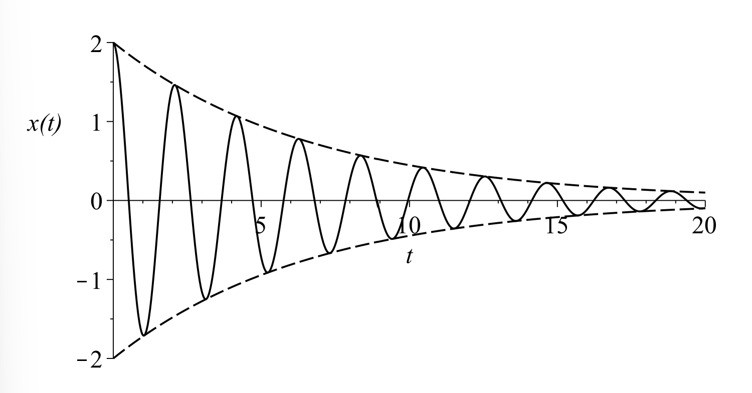
In this case we have complex conjugate roots. We can write \(\alpha=-b / 2 m\) and \(\beta=\sqrt{4 m k-b^{2}} / 2 m .\) Then the solution is
\(x(t)=e^{\alpha t}\left(c_{1} \cos \beta t+c_{2} \sin \beta t\right)\)
These solutions exhibit oscillations due to the trigonometric functions, but we see that the amplitude may decay in time due the overall factor of \(e^{\alpha t}\) when \(\alpha<0 .\) Consider the case that the initial conditions give \(c_{1}=A\) and \(c_{2}=0 .\) (When is this?) Then, the solution, \(x(t)=A e^{\alpha t} \cos \beta t\), looks like the plot in Figure \(\PageIndex{13}.\)