
2.4: Forced Systems
- Page ID
- 91054

ALL OF THE SYSTEMS PRESENTED at the beginning of the last section exhibit the same general behavior when a damping term is present. An additional term can be added that might cause even more complicated behavior. In the case of LRC circuits, we have seen that the voltage source makes the system nonhomogeneous. It provides what is called a source term. Such terms can also arise in the mass-spring and pendulum systems. One can drive such systems by periodically pushing the mass, or having the entire system moved, or impacted by an outside force. Such systems are called forced, or driven.
Typical systems in physics can be modeled by nonhomogeneous second order equations. Thus, we want to find solutions of equations of the form
\[L y(x)=a(x) y^{\prime \prime}(x)+b(x) y^{\prime}(x)+c(x) y(x)=f(x) \label{2.43} \]
As noted in Section 2.1, one solves this equation by finding the general solution of the homogeneous problem,
\(L y_{h}=0\)
and a particular solution of the nonhomogeneous problem,
\(L y_{p}=f .\)
Then, the general solution of Equation \(2.1.1\) is simply given as \(y=y_{h}+y_{p}\).
So far, we only know how to solve constant coefficient, homogeneous equations. So, by adding a nonhomogeneous term to such equations we will need to find the particular solution to the nonhomogeneous equation.
We could guess a solution, but that is not usually possible without a little bit of experience. So, we need some other methods. There are two main methods. In the first case, the Method of Undetermined Coefficients, one makes an intelligent guess based on the form of \(f(x)\). In the second method, one can systematically developed the particular solution. We will come back to the Method of Variation of Parameters and we will also introduce the powerful machinery of Green’s functions later in this section.
Method of Undetermined Coefficients
LET’S SOLVE A SIMPLE DIFFERENTIAL EQUATION highlighting how we can handle nonhomogeneous equations.
Consider the equation
\[y^{\prime \prime}+2 y^{\prime}-3 y=4 \nonumber \]
The first step is to determine the solution of the homogeneous equation. Thus, we solve
\[y_{h}^{\prime \prime}+2 y_{h}^{\prime}-3 y_{h}=0 \nonumber \]
The characteristic equation is \(r^{2}+2 r-3=0 .\) The roots are \(r=1,-3\). So, we can immediately write the solution
\(y_{h}(x)=c_{1} e^{x}+c_{2} e^{-3 x}\)
The second step is to find a particular solution of Equation \(\PageIndex{2}\). What possible function can we insert into this equation such that only a 4 remains? If we try something proportional to \(x\), then we are left with a linear function after inserting \(x\) and its derivatives. Perhaps a constant function you might think. \(y=4\) does not work. But, we could try an arbitrary constant, \(y=A\).
Let’s see. Inserting \(y=A\) into Equation \(\PageIndex{2}\), we obtain
\(-3 A=4\)
Ah ha! We see that we can choose \(A=-\dfrac{4}{3}\) and this works. So, we have a particular solution, \(y_{p}(x)=-\dfrac{4}{3}\). This step is done.
Combining the two solutions, we have the general solution to the original nonhomogeneous equation Equation \(\PageIndex{2}\). Namely,
\(y(x)=y_{h}(x)+y_{p}(x)=c_{1} e^{x}+c_{2} e^{-3 x}-\dfrac{4}{3}\)
Insert this solution into the equation and verify that it is indeed a solution. If we had been given initial conditions, we could now use them to determine the arbitrary constants.
What if we had a different source term? Consider the equation
\[y^{\prime \prime}+2 y^{\prime}-3 y=4 x \nonumber \]
The only thing that would change is the particular solution. So, we need a guess.
We know a constant function does not work by the last example. So, let’s try \(y_{p}=A x\). Inserting this function into Equation \(\PageIndex{4}\), we obtain
\(2 A-3 A x=4 x\)
Picking \(A=-4 / 3\) would get rid of the \(x\) terms, but will not cancel everything. We still have a constant left. So, we need something more general.
Let’s try a linear function, \(y_{p}(x)=A x+B\). Then we get after substitution into Equation \(\PageIndex{4}\)
\[2 A-3(A x+B)=4 x \nonumber \]
Equating the coefficients of the different powers of \(x\) on both sides, we find a system of equations for the undetermined coefficients:
\[ \begin{array}{r} 2 A-3 B=0 \\ -3 A=4 \end{array}\label{2.47} \]
These are easily solved to obtain
\[ \begin{aligned} A &=-\dfrac{4}{3} \\ B &=\dfrac{2}{3} A=-\dfrac{8}{9} \end{aligned}\label{48} \]
So, the particular solution is
\(y_{p}(x)=-\dfrac{4}{3} x-\dfrac{8}{9}\)
This gives the general solution to the nonhomogeneous problem as
\(y(x)=y_{h}(x)+y_{p}(x)=c_{1} e^{x}+c_{2} e^{-3 x}-\dfrac{4}{3} x-\dfrac{8}{9}\)
There are general forms that you can guess based upon the form of the driving term, \(f(x)\). Some examples are given in Table \(\PageIndex{1}\). More general applications are covered in a standard text on differential equations. However, the procedure is simple. Given \(f(x)\) in a particular form, you make an appropriate guess up to some unknown parameters, or coefficients. Inserting the guess leads to a system of equations for the unknown coefficients. Solve the system and you have the solution. This solution is then added to the general solution of the homogeneous differential equation.
| \(f(x)\) | Guess |
|
\(a_{n} x^{n}+a_{n-1} x^{n-1}+\cdots+a_{1} x+a_{0}\) \(a e^{b x}\) \(a \cos \omega x+b \sin \omega x\) |
\(A_{n} x^{n}+A_{n-1} x^{n-1}+\cdots+A_{1} x+A_{0}\) \(A e^{b x}\) \(A \cos \omega x+B \sin \omega x\) |
Solve
\[y^{\prime \prime}+2 y^{\prime}-3 y=2 e^{-3 x} \nonumber \]
According to the above, we would guess a solution of the form \(y_{p}=A e^{-3 x} .\) Inserting our guess, we find
\(0=2 e^{-3 x}\)
Oops! The coefficient, \(A\), disappeared! We cannot solve for it. What went wrong?
The answer lies in the general solution of the homogeneous problem. Note that \(e^{x}\) and \(e^{-3 x}\) are solutions to the homogeneous problem. So, a multiple of \(e^{-3 x}\) will not get us anywhere. It turns out that there is one further modification of the method. If the driving term contains terms that are solutions of the homogeneous problem, then we need to make a guess consisting of the smallest possible power of \(x\) times the function which is no longer a solution of the homogeneous problem. Namely, we guess \(y_{p}(x)=A x e^{-3 x}\) and differentiate this guess to obtain the derivatives \(y_{p}^{\prime}=A(1-3 x) e^{-3 x}\) and \(y_{p}^{\prime \prime}=A(9 x-6) e^{-3 x}\)
Inserting these derivatives into the differential equation, we obtain
\([(9 x-6)+2(1-3 x)-3 x] A e^{-3 x}=2 e^{-3 x}\)
Comparing coefficients, we have
\(-4 A=2\)
So, \(A=-1 / 2\) and \(y_{p}(x)=-\dfrac{1}{2} x e^{-3 x}\). Thus, the solution to the problem is
\(y(x)=\left(2-\dfrac{1}{2} x\right) e^{-3 x}\)
Modified Method of Undetermined Coefficients
In general, if any term in the guess \(y_{p}(x)\) is a solution of the homogeneous equation, then multiply the guess by \(x^{k}\), where \(k\) is the smallest positive integer such that no term in \(x^{k} y_{p}(x)\) is a solution of the homogeneous problem.
2.4.2: Periodically Forced Oscillations
A SPECIAL TYPE OF FORCING is periodic forcing. Realistic oscillations will dampen and eventually stop if left unattended. For example, mechanical clocks are driven by compound or torsional pendula and electric oscillators are often designed with the need to continue for long periods of time. However, they are not perpetual motion machines and will need a periodic injection of energy. This can be done systematically by adding periodic forcing. Another simple example is the motion of a child on a swing in the park. This simple damped pendulum system will naturally slow down to equilibrium (stopped) if left alone. However, if the child pumps energy into the swing at the right time, or if an adult pushes the child at the right time, then the amplitude of the swing can be increased.
There are other systems, such as airplane wings and long bridge spans, in which external driving forces might cause damage to the system. A well know example is the wind induced collapse of the Tacoma Narrows Bridge due to strong winds. Of course, if one is not careful, the child in the last example might get too much energy pumped into the system causing a similar failure of the desired motion.
The Tacoma Narrows Bridge opened in Washington State (U.S.) in mid \(1940 .\) However, in November of the same year the winds excited a transverse mode of vibration, which eventually (in a few hours) lead to large amplitude oscillations and then collapse.
While there are many types of forced systems, and some fairly complicated, we can easily get to the basic characteristics of forced oscillations by modifying the mass-spring system by adding an external, time-dependent, driving force. Such as system satisfies the equation
\[m \ddot{x}+\dot{b(x)}+k x=F(t) \nonumber \]
where \(m\) is the mass, \(b\) is the damping constant, \(k\) is the spring constant, and \(F(t)\) is the driving force. If \(F(t)\) is of simple form, then we can employ the Method of Undetermined Coefficients. Since the systems we have considered so far are similar, one could easily apply the following to pendula or circuits.
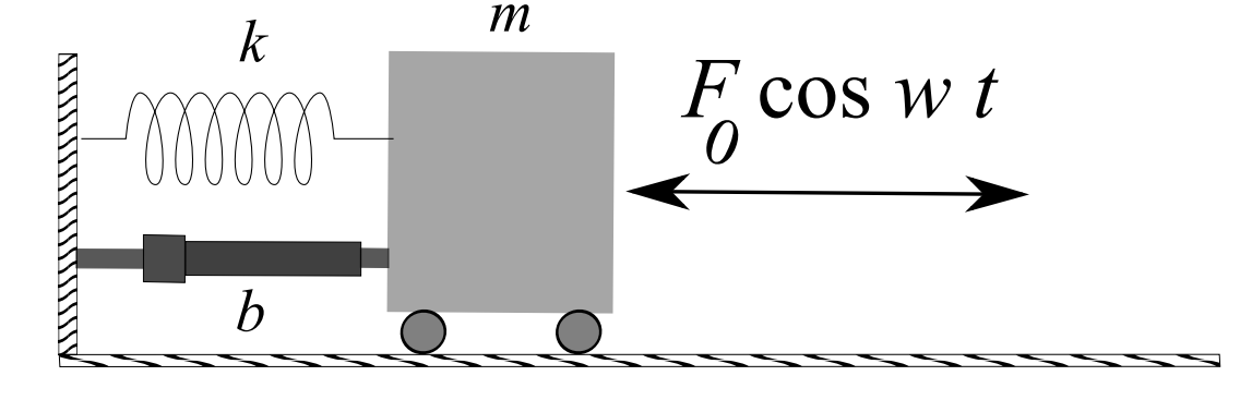
As the damping term only complicates the solution, we will consider the simpler case of undamped motion and assume that \(b=0\). Furthermore, we will introduce a sinusoidal driving force, \(F(t)=F_{0} \cos \omega t\) in order to study periodic forcing. This leads to the simple periodically driven mass on a spring system
\[m \ddot{x}+k x=F_{0} \cos \omega t . \nonumber \]
In order to find the general solution, we first obtain the solution to the homogeneous problem,
\(x_{h}=c_{1} \cos \omega_{0} t+c_{2} \sin \omega_{0} t\)
where \(\omega_{0}=\sqrt{\dfrac{k}{m}} .\) Next, we seek a particular solution to the nonhomogeneous problem. We will apply the Method of Undetermined Coefficients.
A natural guess for the particular solution would be to use \(x_{p}=A \cos \omega t+B \sin \omega t\). However, recall that the guess should not be a solution of the homogeneous problem. Comparing \(x_{p}\) with \(x_{h}\), this would hold if \(\omega \neq \omega_{0} .\) Otherwise, one would need to use the Modified Method of Undetermined Coefficients as described in the last section. So, we have two cases to consider.
Dividing through by the mass, we solve the simple driven system, \(\ddot{x}+\omega_{0}^{2} x=\dfrac{F_{0}}{m} \cos \omega t\)
Solve \(\ddot{x}+\omega_{0}^{2} x=\dfrac{F_{0}}{m} \cos \omega t\), for \(\omega \neq \omega_{0} .\)
In this case we continue with the guess \(x_{p}=A \cos \omega t+B \sin \omega t\).
Since there is no damping term, one quickly finds that \(B=0 .\) Inserting \(x_{p}=A \cos \omega t\) into the differential equation, we find that
\(\left(-\omega^{2}+\omega_{0}^{2}\right) A \cos \omega t=\dfrac{F_{0}}{m} \cos \omega t\)
Solving for A, we obtain
\(A=\dfrac{F_{0}}{m\left(\omega_{0}^{2}-\omega^{2}\right)}\)
The general solution for this case is thus,
\[x(t)=c_{1} \cos \omega_{0} t+c_{2} \sin \omega_{0} t+\dfrac{F_{0}}{m\left(\omega_{0}^{2}-\omega^{2}\right)} \cos \omega t \nonumber \]
Solve \(\ddot{x}+\omega_{0}^{2} x=\dfrac{F_{0}}{m} \cos \omega_{0} t\).
In this case, we need to employ the Modified Method of Undetermined Coefficients. So, we make the guess \(x_{p}=A \cos \omega_0 t+B \sin \omega_0 t\). Since there is no damping term, one finds that A = 0. Inserting the guess in to the differential equation, we find that
\(B=\dfrac{F_{0}}{2 m \omega_{0}}\),
or the general solution is
\[x(t)=c_{1} \cos \omega_{0} t+c_{2} \sin \omega_{0} t+\dfrac{F_{0}}{2 m \omega} t \sin \omega t \nonumber \]
The general solution to the problem is thus
\[ x(t)=c_{1} \cos \omega_{0} t+c_{2} \sin \omega_{0} t+ \begin{cases}\dfrac{F_{0}}{m\left(\omega_{0}^{2}-\omega^{2}\right)} \cos \omega t, & \omega \neq \omega_{0} \\ \dfrac{F_{0}}{2 m \omega_{0}} t \sin \omega_{0} t, & \omega=\omega_{0}\end{cases} \label{2.54} \]
Special cases of these solutions provide interesting physics, which can be explored by the reader in the homework. In the case that \(\omega=\omega_{0}\), we see that the solution tends to grow as \(t\) gets large. This is what is called a resonance. Essentially, one is driving the system at its natural frequency. As the system is moving to the left, one pushes it to the left. If it is moving to the right, one is adding energy in that direction. This forces the amplitude of oscillation to continue to grow until the system breaks. An example of such an oscillation is shown in Figure \(\PageIndex{2}\).
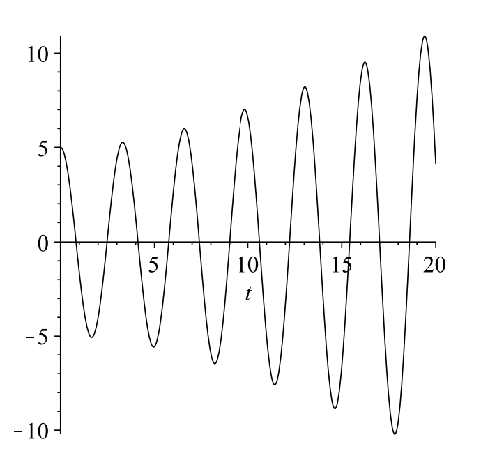 Figure \(\PageIndex{2}\): Plot of \(x(t)=5 \cos 2 t+\dfrac{1}{2} t \sin 2 t\), a solution of \(\ddot{x}+4 x=2 \cos 2 t\) showing resonance.
 In the case that \(\omega \neq \omega_{0}\), one can rewrite the solution in a simple form. Let’s choose the initial conditions that \(c_{1}=-F_{0} /\left(m\left(\omega_{0}^{2}-\omega^{2}\right)\right), c_{2}=0 .\) Then one has (see Problem 13)
\[x(t)=\dfrac{2 F_{0}}{m\left(\omega_{0}^{2}-\omega^{2}\right)} \sin \dfrac{\left(\omega_{0}-\omega\right) t}{2} \sin \dfrac{\left(\omega_{0}+\omega\right) t}{2} \nonumber \]
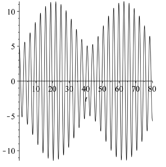
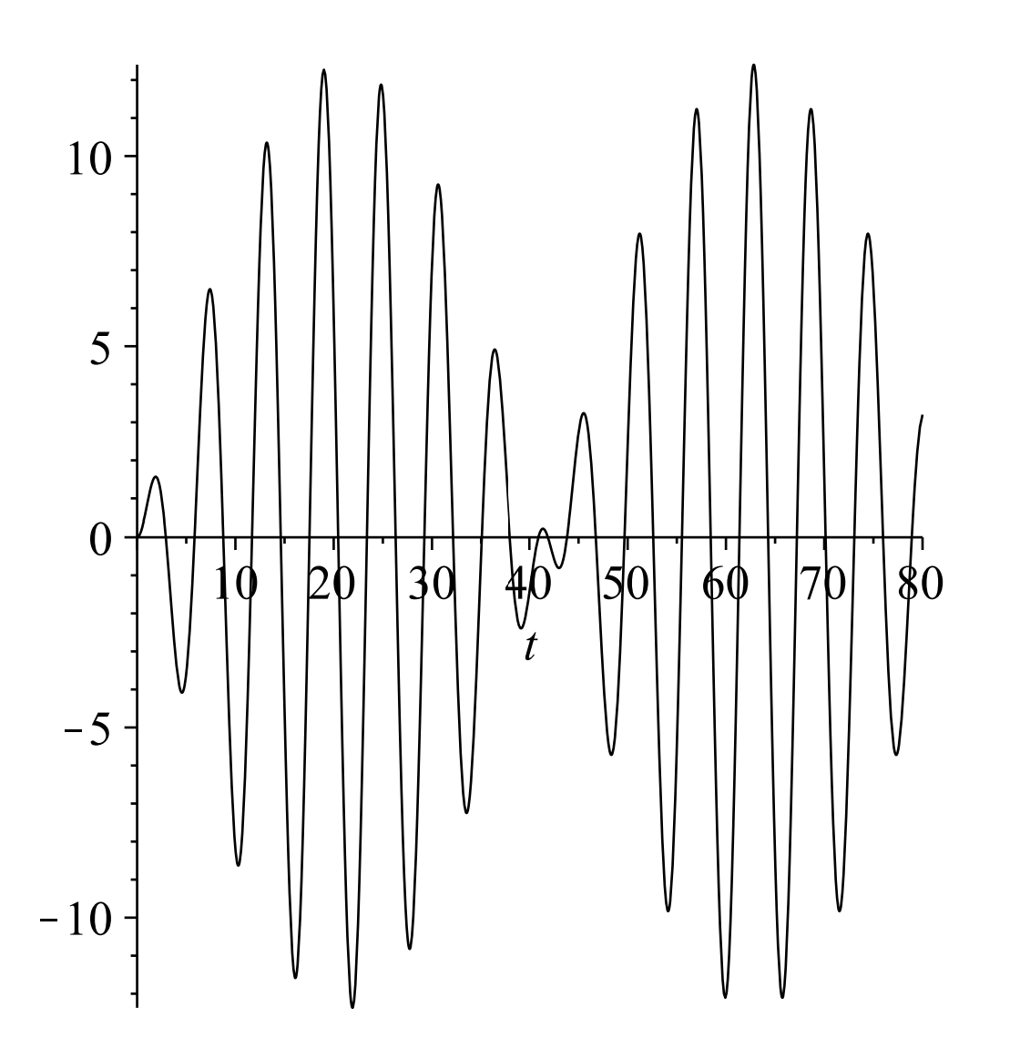
For values of \(\omega\) near \(\omega_{0}\), one finds the solution consists of a rapid oscillation, due to the \(\sin \dfrac{\left(\omega_{0}+\omega\right) t}{2}\) factor, with a slowly varying amplitude, \(\dfrac{2 F_{0}}{m\left(\omega_{0}^{2}-\omega^{2}\right)} \sin \dfrac{\left(\omega_{0}-\omega\right) t}{2} .\) The reader can investigate this solution.
This slow variation is called a beat and the beat frequency is given by \(f=\) \(\dfrac{\left|\omega_{0}-\omega\right|}{4 \pi} .\) In Figure \(\PageIndex{3}\) we see the high frequency oscillations are contained by the lower beat frequency, \(f=\dfrac{0.15}{4 \pi} \mathrm{s}\). This corresponds to a period of \(T=1 / f \approx 83.7 \mathrm{~Hz}\), which looks about right from the figure.
Solve \(\ddot{x}+x=2 \cos \omega t, x(0)=0, \dot{x}(0)=0\), for \(\omega=\) \(1,1.15 .\) For each case, we need the solution of the homogeneous problem,
\(x_{h}(t)=c_{1} \cos t+c_{2} \sin t .\)
The particular solution depends on the value of \(\omega\).
For \(\omega=1\), the driving term, \(2 \cos \omega t\), is a solution of the homogeneous problem. Thus, we assume
\(x_{p}(t)=A t \cos t+B t \sin t .\)
Inserting this into the differential equation, we find \(A=0\) and \(B=1\). So, the general solution is
\(x(t)=c_{1} \cos t+c_{2} \sin t+t \sin t\)
Imposing the initial conditions, we find
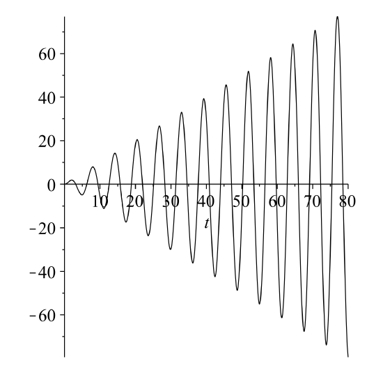
\(x(t)=t \sin t\)
This solution is shown in Figure \(\PageIndex{4}\).
For \(\omega=1.15\), the driving term, \(2 \cos \omega 1.15 t\), is not a solution of the homogeneous problem. Thus, we assume
\(x_{p}(t)=A \cos 1.15 t+B \sin 1.15 t\)
Inserting this into the differential equation, we find \(A=-\dfrac{800}{129}\) and \(B=0 .\) So, the general solution is
\(x(t)=c_{1} \cos t+c_{2} \sin t-\dfrac{800}{129} \cos t\)
Imposing the initial conditions, we find
\(x(t)=\dfrac{800}{129}(\cos t-\cos 1.15 t)\)
This solution is shown in Figure \(\PageIndex{5}\). The beat frequency in this case is the same as with Figure \(\PageIndex{3}\).
Reduction of Order for Nonhomogeneous Equations
The Method of Reduction of Order is also useful for solving nonhomogeneous problems. In this case if we know one solution of the homogeneous problem, then we can use it to obtain a particular solution of the nonhomogenous problem. For example, consider the nonhomogeneous differential equation
\[a(x) y^{\prime \prime}(x)+b(x) y^{\prime}(x)+c(x) y(x)=f(x) \nonumber \]
Let's assume \(y_{1}(x)\) satisfies the homogeneous differential equation
\[a(x) y_{1}^{\prime \prime}(x)+b(x) y_{1}^{\prime}(x)+c(x) y_{1}(x)=0 \nonumber \]
The, we seek a particular solution, \(y_{p}(x)=v(x) y_{1}(x)\) Its derivatives are given by
\(\begin{aligned} y_{p}^{\prime} &=\left(v y_{1}\right)^{\prime} \\ &=v^{\prime} y_{1}+v y_{1}^{\prime} \\ y_{p}^{\prime \prime} &=\left(v^{\prime} y_{1}+v y_{1}^{\prime}\right)^{\prime} \\ &=v^{\prime \prime} y_{1}+2 v^{\prime} y_{1}^{\prime}+v y_{1}^{\prime \prime} \end{aligned} \)
Substituting \(y_{p}\) and its derivatives into the differential equation, we have
\(\begin{aligned} f &=a y_{p}^{\prime \prime}+b y_{p}^{\prime}+c y_{p} \\ &=a\left(v^{\prime \prime} y_{1}+2 v^{\prime} y_{1}^{\prime}+v y_{1}^{\prime \prime}\right)+b\left(v^{\prime} y_{1}+v y_{1}^{\prime}\right)+c v y_{1} \\ &=a v^{\prime \prime} y_{1}+2 a v^{\prime} y_{1}^{\prime}+b v^{\prime} y_{1}+v\left[a y_{1}^{\prime \prime}+b y_{1}^{\prime}+c y_{1}\right] \\ &=a v^{\prime \prime} y_{1}+2 a v^{\prime} y_{1}^{\prime}+b v^{\prime} y_{1} \end{aligned}\)
Therefore, \(v(x)\) satisfies the second order equation
\(a(x) y(x) v^{\prime \prime}(x)+\left[2 a(x) y_{1}^{\prime}(x)+b(x) y_{1}(x)\right] v^{\prime}(x)=f(x)\)
Letting \(z=v^{\prime}\), we see that we have the linear first order equation for \(z(x)\) :
\[\left.a(x) y_{(} x\right) z^{\prime}(x)+\left[2 a(x) y_{1}^{\prime}(x)+b(x) y_{1}(x)\right] z(x)=f(x) \nonumber \]
Use the Method of Reduction of Order to solve \(y^{\prime \prime}+\) \(y=\sec x .\)
Solutions of the homogeneous equation, \(y^{\prime \prime}+y=0\) are \(\sin x\) and \(\cos x .\) We can choose either to begin using the Method of Reduction of Order. Let’s take \(y_{p}=v \cos x .\) Its derivatives are given by
\(\begin{aligned} y_{p}^{\prime} &=(v \cos x)^{\prime} \\ &=v^{\prime} \cos x-v \sin x \\ y_{p}^{\prime \prime} &=\left(v^{\prime} \cos x-v \sin x\right)^{\prime} \\ &=v^{\prime \prime} \cos x-2 v^{\prime} \sin x-v \cos x \end{aligned}\)
Substituting into the nonhomogeneous equation, we have
\(\begin{aligned} \sec x &=y_{p}^{\prime \prime}+y_{p} \\ &=v^{\prime \prime} \cos x-2 v^{\prime} \sin x-v \cos x+v \cos x \\ &=v^{\prime \prime} \cos x-2 v^{\prime} \sin x \end{aligned}\)
Letting \(v^{\prime}=z\), we have the linear first order differential equation
\((\cos x) z^{\prime}-(2 \sin x) z=\sec x\)
Rewriting the equation as,
\(z^{\prime}-(2 \tan x) z=\sec ^{2} x\)
Multiplying by the integrating factor,
\(\begin{aligned} \mu(x) &=-\exp \int^{x} 2 \tan \xi d \xi \\ &=-\exp 2 \ln |\sec x| \\ &=\cos ^{2} x \end{aligned}\)
we obtain
\(\left(z \cos ^{2} x\right)^{\prime}=1\)
Integrating,
\(v^{\prime}=z=x \sec ^{2} x\)
This can be integrated using integration by parts (letting \(U=x\) and \(V=\tan x)\) :
\(\begin{aligned} v &=\int x \sec ^{2} x d x \\ &=x \tan x-\int \tan x d x \\ &=x \tan x-\ln |\sec x| \end{aligned}\)
We now have enough to write out the solution. The particular solution is given by
\(\begin{aligned} y_{p} &=v y_{1} \\ &=(x \tan x-\ln |\sec x|) \cos x \\ &=x \sin x+\cos x \ln |\cos x| \end{aligned}\)
The general solution is then
\(y(x)=c_{1} \cos x+c_{2} \sin x+x \sin x+\cos x \ln |\cos x|\)
Method of Variation of Parameters
A MORE SYSTEMATIC WAY to find particular solutions is through the use of the Method of Variation of Parameters. The derivation is a little detailed and the solution is sometimes messy, but the application of the method is straight forward if you can do the required integrals. We will first derive the needed equations and then do some examples.
We begin with the nonhomogeneous equation. Let’s assume it is of the standard form
\[a(x) y^{\prime \prime}(x)+b(x) y^{\prime}(x)+c(x) y(x)=f(x) \nonumber \]
We know that the solution of the homogeneous equation can be written in terms of two linearly independent solutions, which we will call \(y_{1}(x)\) and \(y_{2}(x):\)
\(y_{h}(x)=c_{1} y_{1}(x)+c_{2} y_{2}(x)\)
Replacing the constants with functions, then we no longer have a solution to the homogeneous equation. Is it possible that we could stumble across the right functions with which to replace the constants and somehow end up with \(f(x)\) when inserted into the left side of the differential equation? It turns out that we can.
So, let’s assume that the constants are replaced with two unknown functions, which we will call \(c_{1}(x)\) and \(c_{2}(x)\). This change of the parameters is where the name of the method derives. Thus, we are assuming that a particular solution takes the form
\[y_{p}(x)=c_{1}(x) y_{1}(x)+c_{2}(x) y_{2}(x). \nonumber \]
We assume the nonhomogeneous equation has a particular solution of the form \(y_{p}(x)=c_{1}(x) y_{1}(x)+c_{2}(x) y_{2}(x)\)
If this is to be a solution, then insertion into the differential equation should make the equation hold. To do this we will first need to compute some derivatives.
The first derivative is given by
\[y_{p}^{\prime}(x)=c_{1}(x) y_{1}^{\prime}(x)+c_{2}(x) y_{2}^{\prime}(x)+c_{1}^{\prime}(x) y_{1}(x)+c_{2}^{\prime}(x) y_{2}(x) \nonumber \]
Next we will need the second derivative. But, this will yield eight terms. So, we will first make a simplifying assumption. Let’s assume that the last two terms add to zero:
\[c_{1}^{\prime}(x) y_{1}(x)+c_{2}^{\prime}(x) y_{2}(x)=0 \nonumber \]
It turns out that we will get the same results in the end if we did not assume this. The important thing is that it works!
Under the assumption the first derivative simplifies to
\[y_{p}^{\prime}(x)=c_{1}(x) y_{1}^{\prime}(x)+c_{2}(x) y_{2}^{\prime}(x) \nonumber \]
The second derivative now only has four terms:
\[y_{p}^{\prime}(x)=c_{1}(x) y_{1}^{\prime \prime}(x)+c_{2}(x) y_{2}^{\prime \prime}(x)+c_{1}^{\prime}(x) y_{1}^{\prime}(x)+c_{2}^{\prime}(x) y_{2}^{\prime}(x) \nonumber \]
Now that we have the derivatives, we can insert the guess into the differential equation. Thus, we have
\[ \begin{aligned} f(x)=& a(x)\left[c_{1}(x) y_{1}^{\prime \prime}(x)+c_{2}(x) y_{2}^{\prime \prime}(x)+c_{1}^{\prime}(x) y_{1}^{\prime}(x)+c_{2}^{\prime}(x) y_{2}^{\prime}(x)\right] \\ &+b(x)\left[c_{1}(x) y_{1}^{\prime}(x)+c_{2}(x) y_{2}^{\prime}(x)\right] \\ &+c(x)\left[c_{1}(x) y_{1}(x)+c_{2}(x) y_{2}(x)\right] \end{aligned} \label{2.64} \]
Regrouping the terms, we obtain
\[ \begin{aligned} f(x)=& c_{1}(x)\left[a(x) y_{1}^{\prime \prime}(x)+b(x) y_{1}^{\prime}(x)+c(x) y_{1}(x)\right] \\ &+c_{2}(x)\left[a(x) y_{2}^{\prime \prime}(x)+b(x) y_{2}^{\prime}(x)+c(x) y_{2}(x)\right] \\ &+a(x)\left[c_{1}^{\prime}(x) y_{1}^{\prime}(x)+c_{2}^{\prime}(x) y_{2}^{\prime}(x)\right] \end{aligned} \label{2.65} \]
Note that the first two rows vanish since \(y_{1}\) and \(y_{2}\) are solutions of the homogeneous problem. This leaves the equation
\[f(x)=a(x)\left[c_{1}^{\prime}(x) y_{1}^{\prime}(x)+c_{2}^{\prime}(x) y_{2}^{\prime}(x)\right] \nonumber \]
which can be rearranged as
\[c_{1}^{\prime}(x) y_{1}^{\prime}(x)+c_{2}^{\prime}(x) y_{2}^{\prime}(x)=\dfrac{f(x)}{a(x)} \nonumber \]
In order to solve the differential equation \(L y=f\), we assume \(y_{p}(x)=c_{1}(x) y_{1}(x)+c_{2}(x) y_{2}(x)\) for \(L y_{1,2}=0\). Then, one need only solve a simple system of Equation \(\PageIndex{25}\).
In summary, we have assumed a particular solution of the form
\(y_{p}(x)=c_{1}(x) y_{1}(x)+c_{2}(x) y_{2}(x)\)
This is only possible if the unknown functions \(c_{1}(x)\) and \(c_{2}(x)\) satisfy the system of equations
\[\begin{aligned} & c_{1}^{\prime}(x) y_{1}(x)+c_{2}^{\prime}(x) y_{2}(x)=0 \\ & c_{1}^{\prime}(x) y_{1}^{\prime}(x)+c_{2}^{\prime}(x) y_{2}^{\prime}(x)=& \dfrac{f(x)}{a(x)} \end{aligned}\label{2.67} \]
It is standard to solve this system for the derivatives of the unknown functions and then present the integrated forms. However, one could just as easily start from this system and solve the system for each problem encountered.
System \(\PageIndex{25}\) can be solved as \(\begin{aligned} c_{1}^{\prime}(x)=-\dfrac{f y_{2}}{a W\left(y_{1}, y_{2}\right)} \\ c_{1}^{\prime}(x)=\dfrac{f y_{1}}{a W\left(y_{1}, y_{2}\right)} \end{aligned}\) where \(W\left(y_{1}, y_{2}\right)=y_{1} y_{2}^{\prime}-y_{1}^{\prime} y_{2}\) is the Wronskian. We use this solution in the next section.
Find the general solution of the nonhomogeneous problem: \(y^{\prime \prime}-y=e^{2 x}\).
The general solution to the homogeneous problem \(y_{h}^{\prime \prime}-y_{h}=0\) is
\(y_{h}(x)=c_{1} e^{x}+c_{2} e^{-x}\)
In order to use the Method of Variation of Parameters, we seek a solution of the form
\(y_{p}(x)=c_{1}(x) e^{x}+c_{2}(x) e^{-x}\)
We find the unknown functions by solving the system in Equation \(\PageIndex{25}\), which in this case becomes
\[\begin{equation} \begin{aligned} &c_{1}^{\prime}(x) e^{x}+c_{2}^{\prime}(x) e^{-x}=0 \\ &c_{1}^{\prime}(x) e^{x}-c_{2}^{\prime}(x) e^{-x}=e^{2 x} \end{aligned} \end{equation}\label{2.68} \]
Adding these equations we find that
\(2 c_{1}^{\prime} e^{x}=e^{2 x} \rightarrow c_{1}^{\prime}=\dfrac{1}{2} e^{x}\)
Solving for \(c_{1}(x)\) we find
\(c_{1}(x)=\dfrac{1}{2} \int e^{x} d x=\dfrac{1}{2} e^{x}\)
Subtracting the equations in the system yields
\(2 c_{2}^{\prime} e^{-x}=-e^{2 x} \rightarrow c_{2}^{\prime}=-\dfrac{1}{2} e^{3 x}\)
Thus,
\(c_{2}(x)=-\dfrac{1}{2} \int e^{3 x} d x=-\dfrac{1}{6} e^{3 x}\)
The particular solution is found by inserting these results into \(y_{p}\) :
\[\begin{equation} \begin{aligned} y_{p}(x) &=c_{1}(x) y_{1}(x)+c_{2}(x) y_{2}(x) \\ &=\left(\dfrac{1}{2} e^{x}\right) e^{x}+\left(-\dfrac{1}{6} e^{3 x}\right) e^{-x} \\ &=\dfrac{1}{3} e^{2 x} \end{aligned} \end{equation}\label{2.69} \]
Thus, we have the general solution of the nonhomogeneous problem as
\(y(x)=c_{1} e^{x}+c_{2} e^{-x}+\dfrac{1}{3} e^{2 x}\)
Now consider the problem: \(y^{\prime \prime}+4 y=\sin x\).
The solution to the homogeneous problem is
\[y_{h}(x)=c_{1} \cos 2 x+c_{2} \sin 2 x . \nonumber \]
We now seek a particular solution of the form
\(y_{h}(x)=c_{1}(x) \cos 2 x+c_{2}(x) \sin 2 x .\)
We let \(y_{1}(x)=\cos 2 x\) and \(y_{2}(x)=\sin 2 x, a(x)=1, f(x)=\sin x\) in Equation \(\PageIndex{25}\):
\[\begin{aligned} c_{1}^{\prime}(x) \cos 2 x+c_{2}^{\prime}(x) \sin 2 x &=0 \\ -2 c_{1}^{\prime}(x) \sin 2 x+2 c_{2}^{\prime}(x) \cos 2 x &=\sin x. \end{aligned}\label{2.71} \]
Now, use your favorite method for solving a system of two equations and two unknowns. In this case, we can multiply the first equation by \(2 \sin 2 x\) and the second equation by \(\cos 2 x\). Adding the resulting equations will eliminate the \(c_{1}^{\prime}\) terms. Thus, we have
\(c_{2}^{\prime}(x)=\dfrac{1}{2} \sin x \cos 2 x=\dfrac{1}{2}\left(2 \cos ^{2} x-1\right) \sin x\)
Inserting this into the first equation of the system, we have
\(c_{1}^{\prime}(x)=-c_{2}^{\prime}(x) \dfrac{\sin 2 x}{\cos 2 x}=-\dfrac{1}{2} \sin x \sin 2 x=-\sin ^{2} x \cos x\)
These can easily be solved:
\(\begin{gathered} c_{2}(x)=\dfrac{1}{2} \int\left(2 \cos ^{2} x-1\right) \sin x d x=\dfrac{1}{2}\left(\cos x-\dfrac{2}{3} \cos ^{3} x\right) \\ c_{1}(x)=-\int \sin ^{x} \cos x d x=-\dfrac{1}{3} \sin ^{3} x \end{gathered}\)
The final step in getting the particular solution is to insert these functions into \(y_{p}(x)\). This gives
\[\begin{equation} \begin{aligned} y_{p}(x) &=c_{1}(x) y_{1}(x)+c_{2}(x) y_{2}(x) \\ &=\left(-\dfrac{1}{3} \sin ^{3} x\right) \cos 2 x+\left(\dfrac{1}{2} \cos x-\dfrac{1}{3} \cos ^{3} x\right) \sin x \\ &=\dfrac{1}{3} \sin x \end{aligned}\end{equation}\label{2.72} \]
So, the general solution is
\[y(x)=c_{1} \cos 2 x+c_{2} \sin 2 x+\dfrac{1}{3} \sin x \nonumber \]
2.4.5: Initial Value Green’s Functions
IN THIS SECTION WE WILL INVESTIGATE the solution of initial value problems involving nonhomogeneous differential equations using Green’s functions. Our goal is to solve the nonhomogeneous differential equation
\[a(t) y^{\prime \prime}(t)+b(t) y^{\prime}(t)+c(t) y(t)=f(t) \label{2.74} \]
subject to the initial conditions
\(y(0)=y_{0} \quad y^{\prime}(0)=v_{0}\)
Since we are interested in initial value problems, we will denote the independent variable as a time variable, \(t\).
Equation \(\PageIndex{32}\) can be written compactly as
\(L[y]=f\)
where \(L\) is the differential operator
\(L=a(t) \dfrac{d^{2}}{d t^{2}}+b(t) \dfrac{d}{d t}+c(t)\)
The solution is formally given by
\(y=L^{-1}[f]\)
The inverse of a differential operator is an integral operator, which we seek to write in the form
\(y(t)=\int G(t, \tau) f(\tau) d \tau\)
The function \(G(t, \tau)\) is referred to as the kernel of the integral operator and is called the Green’s function.
The history of the Green’s function dates back to 1828, when George Green published work in which he sought solutions of Poisson’s equation \(\nabla^{2} u=f\) for the electric potential \(u\) defined inside a bounded volume with specified boundary conditions on the surface of the volume. He introduced a function now identified as what Riemann later coined the "Green’s func-tion”. In this section we will derive the initial value Green’s function for ordinary differential equations. Later in the book we will return to boundary value Green’s functions and Green's funcitons for partial differential equations.
George Green (1793-1841), a British mathematical physicist who had little formal education and worked as a miller and a baker, published An Essay on the Application of Mathematical Analysis to the Theories of Electricity and Magnetism in which he not only introduced what is now known as Green’s function, but he also introduced potential theory and Green’s Theorem in his studies of electricity and magnetism. Recently his paper was posted at arXiv.org, arXiv:0807.0088.
In the last section we solved nonhomogeneous equations like Equation \(\PageIndex{32}\) using the Method of Variation of Parameters. Letting,
\[y_{p}(t)=c_{1}(t) y_{1}(t)+c_{2}(t) y_{2}(t) \nonumber \]
we found that we have to solve the system of equations
\[ \begin{aligned} &c_{1}^{\prime}(t) y_{1}(t)+c_{2}^{\prime}(t) y_{2}(t)=0 \\ &c_{1}^{\prime}(t) y_{1}^{\prime}(t)+c_{2}^{\prime}(t) y_{2}^{\prime}(t)=\dfrac{f(t)}{q(t)} \end{aligned} \label{2.76} \]
This system is easily solved to give
\[ \begin{aligned} &c_{1}^{\prime}(t)=-\dfrac{f(t) y_{2}(t)}{a(t)\left[y_{1}(t) y_{2}^{\prime}(t)-y_{1}^{\prime}(t) y_{2}(t)\right]} \\ &c_{2}^{\prime}(t)=\dfrac{f(t) y_{1}(t)}{a(t)\left[y_{1}(t) y_{2}^{\prime}(t)-y_{1}^{\prime}(t) y_{2}(t)\right]} . \end{aligned} \label{2.77} \]
We note that the denominator in these expressions involves the Wronskian of the solutions to the homogeneous problem, which is given by the determinant
\[W\left(y_{1}, y_{2}\right)(t)=\left|\begin{array}{ll} y_{1}(t) & y_{2}(t) \\ y_{1}^{\prime}(t) & y_{2}^{\prime}(t) \end{array}\right| \nonumber \]
When \(y_{1}(t)\) and \(y_{2}(t)\) are linearly independent, then the Wronskian is not zero and we are guaranteed a solution to the above system.
So, after an integration, we find the parameters as
\[ \begin{aligned} c_{1}(t) &=-\int_{t_{0}}^{t} \dfrac{f(\tau) y_{2}(\tau)}{a(\tau) W(\tau)} d \tau \\ c_{2}(t) &=\int_{t_{1}}^{t} \dfrac{f(\tau) y_{1}(\tau)}{a(\tau) W(\tau)} d \tau \end{aligned} \label{2.79} \]
where \(t_{0}\) and \(t_{1}\) are arbitrary constants to be determined from the initial conditions.
Therefore, the particular solution of \(Equation \(\PageIndex{32}\)\) can be written as
\[ y_{p}(t)=y_{2}(t) \int_{t_{1}}^{t} \dfrac{f(\tau) y_{1}(\tau)}{a(\tau) W(\tau)} d \tau-y_{1}(t) \int_{t_{0}}^{t} \dfrac{f(\tau) y_{2}(\tau)}{a(\tau) W(\tau)} d \tau \nonumber \]
We begin with the particular solution Equation \(\PageIndex{37}\) of the nonhomogeneous differential equation Equation \(\PageIndex{32}\). This can be combined with the general solution of the homogeneous problem to give the general solution of the nonhomogeneous differential equation:
\[y_{p}(t)=c_{1} y_{1}(t)+c_{2} y_{2}(t)+y_{2}(t) \int_{t_{1}}^{t} \dfrac{f(\tau) y_{1}(\tau)}{a(\tau) W(\tau)} d \tau-y_{1}(t) \int_{t_{0}}^{t} \dfrac{f(\tau) y_{2}(\tau)}{a(\tau) W(\tau)} d \tau \nonumber \]
However, an appropriate choice of \(t_{0}\) and \(t_{1}\) can be found so that we need not explicitly write out the solution to the homogeneous problem, \(c_{1} y_{1}(t)+c_{2} y_{2}(t) .\) However, setting up the solution in this form will allow us to use \(t_{0}\) and \(t_{1}\) to determine particular solutions which satisfies certain homogeneous conditions. In particular, we will show that Equation \(\PageIndex{38}\) can be written in the form
\[y(t)=c_{1} y_{1}(t)+c_{2} y_{2}(t)+\int_{0}^{t} G(t, \tau) f(\tau) d \tau \nonumber \]
where the function \(G(t, \tau)\) will be identified as the Green’s function.
The goal is to develop the Green’s function technique to solve the initial value problem
\[a(t) y^{\prime \prime}(t)+b(t) y^{\prime}(t)+c(t) y(t)=f(t), \quad y(0)=y_{0}, \quad y^{\prime}(0)=v_{0} \nonumber \]
We first note that we can solve this initial value problem by solving two separate initial value problems. We assume that the solution of the homogeneous problem satisfies the original initial conditions:
\[a(t) y_{h}^{\prime \prime}(t)+b(t) y_{h}^{\prime}(t)+c(t) y_{h}(t)=0, \quad y_{h}(0)=y_{0}, \quad y_{h}^{\prime}(0)=v_{0} \nonumber \]
We then assume that the particular solution satisfies the problem
\[a(t) y_{p}^{\prime \prime}(t)+b(t) y_{p}^{\prime}(t)+c(t) y_{p}(t)=f(t), \quad y_{p}(0)=0, \quad y_{p}^{\prime}(0)=0 \nonumber \]
Since the differential equation is linear, then we know that
\(y(t)=y_{h}(t)+y_{p}(t)\)
is a solution of the nonhomogeneous equation. Also, this solution satisfies the initial conditions:
\(\begin{aligned} &y(0)=y_{h}(0)+y_{p}(0)=y_{0}+0=y_{0} \\ &y^{\prime}(0)=y_{h}^{\prime}(0)+y_{p}^{\prime}(0)=v_{0}+0=v_{0} \end{aligned}\)
Therefore, we need only focus on finding a particular solution that satisfies homogeneous initial conditions. This will be done by finding values for \(t_{0}\) and \(t_{1}\) in Equation \(\PageIndex{37}\) which satisfy the homogeneous initial conditions, \(y_{p}(0)=0\) and \(y_{p}^{\prime}(0)=0\).
First, we consider \(y_{p}(0)=0 .\) We have
\[y_{p}(0)=y_{2}(0) \int_{t_{1}}^{0} \dfrac{f(\tau) y_{1}(\tau)}{a(\tau) W(\tau)} d \tau-y_{1}(0) \int_{t_{0}}^{0} \dfrac{f(\tau) y_{2}(\tau)}{a(\tau) W(\tau)} d \tau \nonumber \]
Here, \(y_{1}(t)\) and \(y_{2}(t)\) are taken to be any solutions of the homogeneous differential equation. Let’s assume that \(y_{1}(0)=0\) and \(y_{2} \neq(0)=0 .\) Then, we have
\[y_{p}(0)=y_{2}(0) \int_{t_{1}}^{0} \dfrac{f(\tau) y_{1}(\tau)}{a(\tau) W(\tau)} d \tau \nonumber \]
We can force \(y_{p}(0)=0\) if we set \(t_{1}=0\).
Now, we consider \(y_{p}^{\prime}(0)=0\). First we differentiate the solution and find that
\[y_{p}^{\prime}(t)=y_{2}^{\prime}(t) \int_{0}^{t} \dfrac{f(\tau) y_{1}(\tau)}{a(\tau) W(\tau)} d \tau-y_{1}^{\prime}(t) \int_{t_{0}}^{t} \dfrac{f(\tau) y_{2}(\tau)}{a(\tau) W(\tau)} d \tau \nonumber \]
since the contributions from differentiating the integrals will cancel. Evaluating this result at \(t=0\), we have
\[y_{p}^{\prime}(0)=-y_{1}^{\prime}(0) \int_{t_{0}}^{0} \dfrac{f(\tau) y_{2}(\tau)}{a(\tau) W(\tau)} d \tau \nonumber \]
Assuming that \(y_{1}^{\prime}(0) \neq 0\), we can set \(t_{0}=0\).
Thus, we have found that
\[ \begin{aligned} y_{p}(x) &=y_{2}(t) \int_{0}^{t} \dfrac{f(\tau) y_{1}(\tau)}{a(\tau) W(\tau)} d \tau-y_{1}(t) \int_{0}^{t} \dfrac{f(\tau) y_{2}(\tau)}{a(\tau) W(\tau)} d \tau \\ &=\int_{0}^{t}\left[\dfrac{y_{1}(\tau) y_{2}(t)-y_{1}(t) y_{2}(\tau)}{a(\tau) W(\tau)}\right] f(\tau) d \tau \end{aligned}\label{2.89} \]
This result is in the correct form and we can identify the temporal, or initial value, Green’s function. So, the particular solution is given as
\[y_{p}(t)=\int_{0}^{t} G(t, \tau) f(\tau) d \tau \nonumber \]
where the initial value Green’s function is defined as
\(G(t, \tau)=\dfrac{y_{1}(\tau) y_{2}(t)-y_{1}(t) y_{2}(\tau)}{a(\tau) W(\tau)}\)
We summarize
Solution of IVP Using the Green’s Function
The solution of the initial value problem,
\(a(t) y^{\prime \prime}(t)+b(t) y^{\prime}(t)+c(t) y(t)=f(t), \quad y(0)=y_{0}, \quad y^{\prime}(0)=v_{0}\)
takes the form
\[y(t)=y_{h}(t)+\int_{0}^{t} G(t, \tau) f(\tau) d \tau \nonumber \]
where
\[G(t, \tau)=\dfrac{y_{1}(\tau) y_{2}(t)-y_{1}(t) y_{2}(\tau)}{a(\tau) W(\tau)} \nonumber \]
is the Green’s function and \(y_{1}, y_{2}, y_{h}\) are solutions of the homogeneous equation satisfying
\(y_{1}(0)=0, y_{2}(0) \neq 0, y_{1}^{\prime}(0) \neq 0, y_{2}^{\prime}(0)=0, y_{h}(0)=y_{0}, y_{h}^{\prime}(0)=v_{0}\)
Solve the forced oscillator problem
\(x^{\prime \prime}+x=2 \cos t, \quad x(0)=4, \quad x^{\prime}(0)=0\)
We first solve the homogeneous problem with nonhomogeneous initial conditions:
\[x_{h}^{\prime \prime}+x_{h}=0, \quad x_{h}(0)=4, \quad x_{h}^{\prime}(0)=0 \nonumber \]
The solution is easily seen to be \(x_{h}(t)=4 \cos t\).
Next, we construct the Green’s function. We need two linearly independent solutions, \(y_{1}(x), y_{2}(x)\), to the homogeneous differential equation satisfying different homogeneous conditions, \(y_{1}(0)=0\) and \(y_{2}^{\prime}(0)=0 .\) The simplest solutions are \(y_{1}(t)=\sin t\) and \(y_{2}(t)=\cos t .\) The Wronskian is found as
\(W(t)=y_{1}(t) y_{2}^{\prime}(t)-y_{1}^{\prime}(t) y_{2}(t)=-\sin ^{2} t-\cos ^{2} t=-1\)
Since \(a(t)=1\) in this problem, we compute the Green’s function,
\[\begin{equation} \begin{aligned} G(t, \tau) &=\dfrac{y_{1}(\tau) y_{2}(t)-y_{1}(t) y_{2}(\tau)}{a(\tau) W(\tau)} \\ &=\sin t \cos \tau-\sin \tau \cos t \\ &=\sin (t-\tau) \end{aligned}\end{equation}\label{2.93} \]
Note that the Green’s function depends on \(t-\tau\). While this is useful in some contexts, we will use the expanded form when carrying out the integration.
We can now determine the particular solution of the nonhomogeneous differential equation. We have
\[\begin{equation} \begin{aligned} x_{p}(t) &=\int_{0}^{t} G(t, \tau) f(\tau) d \tau \\ &=\int_{0}^{t}(\sin t \cos \tau-\sin \tau \cos t)(2 \cos \tau) d \tau \\ &=2 \sin t \int_{0}^{t} \cos ^{2} \tau d \tau-2 \cos t \int_{0}^{t} \sin \tau \cos \tau d \tau \\ &=2 \sin t\left[\dfrac{\tau}{2}+\dfrac{1}{2} \sin 2 \tau\right]_{0}^{t}-2 \cos t\left[\dfrac{1}{2} \sin ^{2} \tau\right]_{0}^{t} \\ &=t \sin t \end{aligned} \end{equation}\label{2.94} \]
Therefore, the solution of the nonhomogeneous problem is the sum of the solution of the homogeneous problem and this particular solution: \(x(t)=4 \cos t+t \sin t\)