4.5: Legendre Polynomials

Legendre Polynomials are one of a set of classical orthogonal polynomials. These polynomials satisfy a second-order linear differential equation. This differential equation occurs naturally in the solution of initial boundary value problems in three dimensions which possess some spherical symmetry. Legendre polynomials, or Legendre functions of the first kind, are solutions of the differential equation

\(^{1}\) Adrien-Marie Legendre (1752-1833) was a French mathematician who made many contributions to analysis and algebra.

\[\left(1-x^{2}\right) y^{\prime \prime}-2 x y^{\prime}+n(n+1) y=0\nonumber \]

In Example 4.4 we found that for n an integer, there are polynomial solutions. The first of these are given by \(P_0(x) = c_0\), \(P_1(x) = c_1x\), and \(P_2(x) = c_2(1 − 3x^2 )\). As the Legendre equation is a linear second-order differential equation, we expect two linearly independent solutions. The second solution, called the Legendre function of the second kind, is given by \(Q_n(x)\) and is not well behaved at \(x = \pm 1\). For example,

\[Q_0(x) = \dfrac{1}{ 2} ln \dfrac{1 + x }{1 − x} \nonumber \]

. We will mostly focus on the Legendre polynomials and some of their properties in this section.

A generalization of the Legendre equation is given by \((1 − x^2 )y'' − 2xy' + [n(n + 1) − \dfrac{m^2 }{1−x^2}] y = 0. \nonumber \]

Solutions to this equation, \(P^m_n(x)\) and \(Q^m_n (x)\), are called the associated Legendre functions of the first and second kind.

4.5.1: Properties of Legendre Polynomials

LEGENDRE POLYNOMIALS BELONG TO THE CLASS Of classical orthogonal polynomials. Members of this class satisfy similar properties. First, we have the Rodrigues Formula for Legendre polynomials:

\[P_{n}(x)=\dfrac{1}{2^{n} n !} \dfrac{d^{n}}{d x^{n}}\left(x^{2}-1\right)^{n}, \quad n \in N_{0} \nonumber \]

(The Rodrigues Formula). From the Rodrigues formula, one can show that \(P_{n}(x)\) is an \(n\)th degree polynomial. Also, for \(n\) odd, the polynomial is an odd function and for \(n\) even, the polynomial is an even function.

Example \(\PageIndex{1}\)

Determine \(P_{2}(x)\) from the Rodrigues Formula:

\[ \begin{aligned} P_{2}(x) &=\dfrac{1}{2^{2} 2 !} \dfrac{d^{2}}{d x^{2}}\left(x^{2}-1\right)^{2} \\ &=\dfrac{1}{8} \dfrac{d^{2}}{d x^{2}}\left(x^{4}-2 x^{2}+1\right) \\ &=\dfrac{1}{8} \dfrac{d}{d x}\left(4 x^{3}-4 x\right) \\ &=\dfrac{1}{8}\left(12 x^{2}-4\right) \\ &=\dfrac{1}{2}\left(3 x^{2}-1\right) \end{aligned} \label{4.52} \]

Note that we get the same result as we found in the last section using orthogonalization.

Table \(\PageIndex{1}\): Tabular computation of the Legendre polynomials using the Rodrigues Formula.

\(n\)	\(\left(x^{2}-1\right)^{n}\)	\(\dfrac{d^{n}}{d x^{n}}\left(x^{2}-1\right)^{n}\)	\(\dfrac{1}{2^{n} n !}\)	\(P_{n}(x)\)
\(\mathrm{O}\)	1	1	1	1
1	\(x^{2}-1\)	\(2 x\)	\(\dfrac{1}{2}\)	\(x\)
2	\(x^{4}-2 x^{2}+1\)	\(12 x^{2}-4\)	\(\dfrac{1}{8}\)	\(\dfrac{1}{2}\left(3 x^{2}-1\right)\)
3	\(x^{6}-3 x^{4}+3 x^{2}-1\)	\(120 x^{3}-72 x\)	\(\dfrac{1}{48}\)	\(\dfrac{1}{2}\left(5 x^{3}-3 x\right)\)

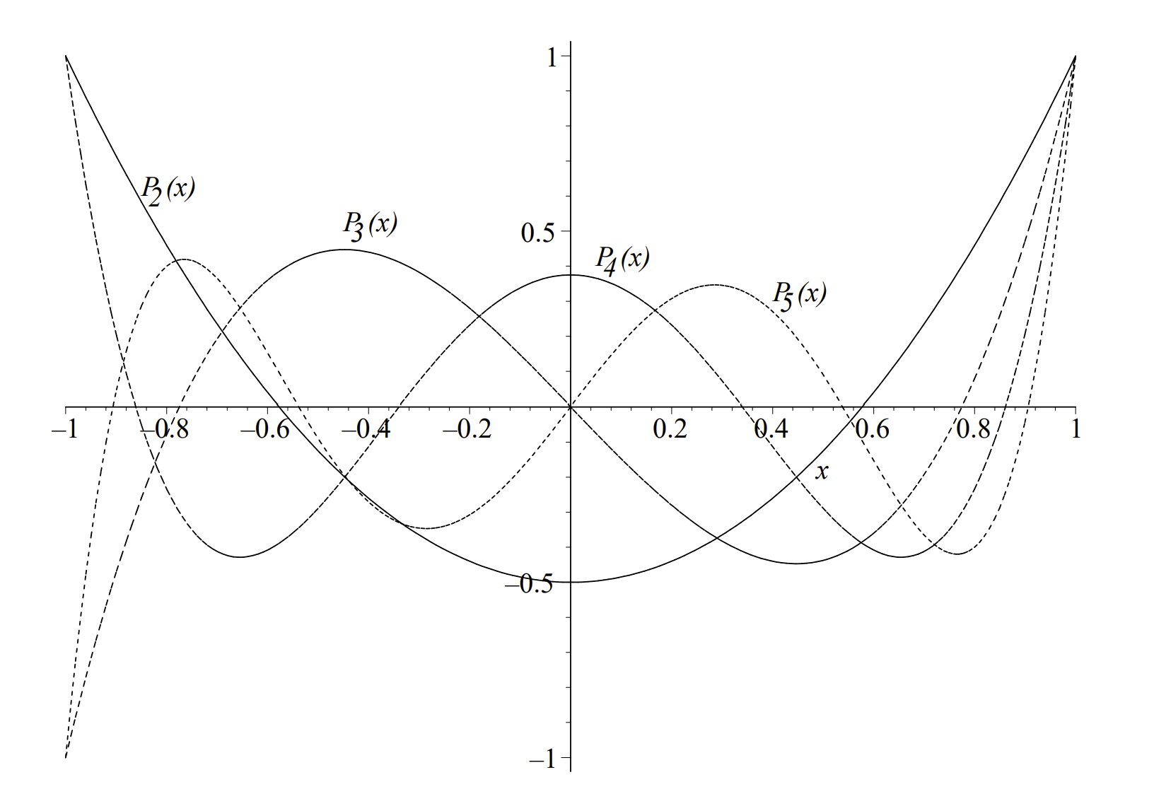
The Three-Term Recursion Formula. The first several Legendre polynomials are given in Table \(\PageIndex{1}\). In Figure \(\PageIndex{1}\) we show plots of these Legendre polynomials.

The classical orthogonal polynomials also satisfy a three-term recursion formula (or, recurrence relation or formula). In the case of the Legendre polynomials, we have

\[(n+1) P_{n+1}(x)=(2 n+1) x P_{n}(x)-n P_{n-1}(x), \quad n=1,2, \ldots \nonumber \]

This can also be rewritten by replacing \(n\) with \(n-1\) as

\[(2 n-1) x P_{n-1}(x)=n P_{n}(x)+(n-1) P_{n-2}(x), \quad n=1,2, \ldots \nonumber \]

Example \(\PageIndex{2}\)

Use the recursion formula to find \(P_{2}(x)\) and \(P_{3}(x)\), given that \(P_{0}(x)=1\) and \(P_{1}(x)=x\).

We first begin by inserting \(n=1\) into Equation \(\PageIndex{3}\):

\[2 P_{2}(x)=3 x P_{1}(x)-P_{0}(x)=3 x^{2}-1. \nonumber \]

Figure \(\PageIndex{1}\): Plots of the Legendre polynomials \(P_2(x)\), \(P_3(x)\), \(P_4(x)\), and \(P_5(x)\).

So, \(P_{2}(x)=\dfrac{1}{2}\left(3 x^{2}-1\right)\)
For \(n=2\), we have

\[ \begin{aligned} 3 P_{3}(x) &=5 x P_{2}(x)-2 P_{1}(x) \\ &=\dfrac{5}{2} x\left(3 x^{2}-1\right)-2 x \\ &=\dfrac{1}{2}\left(15 x^{3}-9 x\right) \end{aligned} \label{4.55} \]

This gives \(P_{3}(x)=\dfrac{1}{2}\left(5 x^{3}-3 x\right).\) These expressions agree with the earlier results.

4.5.2: The Generating Function for Legendre Polynomials

A PROOF OF THE THREE-TERM RECURSION FORMULA can be obtained from the generating function of the Legendre polynomials. Many special functions have such generating functions. In this case, it is given by

\[g(x, t)=\dfrac{1}{\sqrt{1-2 x t+t^{2}}}=\sum_{n=0}^{\infty} P_{n}(x) t^{n}, \quad|x| \leq 1,|t|<1 \nonumber \]

This generating function occurs often in applications. In particular, it arises in potential theory, such as electromagnetic or gravitational potentials. These potential functions are \(\dfrac{1}{r}\) type functions.

Figure \(\PageIndex{2}\): The position vectors used to describe the tidal force on the Earth due to the moon.

For example, the gravitational potential between the Earth and the moon is proportional to the reciprocal of the magnitude of the difference between their positions relative to some coordinate system. An even better example would be to place the origin at the center of the Earth and consider the forces on the non-pointlike Earth due to the moon. Consider a piece of the Earth at position \(\mathbf{r}_{1}\) and the moon at position \(\mathbf{r}_{2}\) as shown in Figure \(\PageIndex{2}\). The tidal potential \(\Phi\) is proportional to

\[\Phi \propto \dfrac{1}{\left|\mathbf{r}_{2}-\mathbf{r}_{1}\right|}=\dfrac{1}{\sqrt{\left(\mathbf{r}_{2}-\mathbf{r}_{1}\right) \cdot\left(\mathbf{r}_{2}-\mathbf{r}_{1}\right)}}=\dfrac{1}{\sqrt{r_{1}^{2}-2 r_{1} r_{2} \cos \theta+r_{2}^{2}}} \nonumber \]

where \(\theta\) is the angle between \(\mathbf{r}_{1}\) and \(\mathbf{r}_{2} .\)

Typically, one of the position vectors is much larger than the other. Let’s assume that \(r_{1} \ll r_{2}\). Then, one can write

\[\Phi \propto \dfrac{1}{\sqrt{r_{1}^{2}-2 r_{1} r_{2} \cos \theta+r_{2}^{2}}}=\dfrac{1}{r_{2}} \dfrac{1}{\sqrt{1-2 \dfrac{r_{1}}{r_{2}} \cos \theta+\left(\dfrac{r_{1}}{r_{2}}\right)^{2}}} \nonumber \]

Now, define \(x=\cos \theta\) and \(t=\dfrac{r_{1}}{r_{2}} .\) We then have that the tidal potential is proportional to the generating function for the Legendre polynomials! So, we can write the tidal potential as

\[\Phi \propto \dfrac{1}{r_{2}} \sum_{n=0}^{\infty} P_{n}(\cos \theta)\left(\dfrac{r_{1}}{r_{2}}\right)^{n} \nonumber \]

The first term in the expansion, \(\dfrac{1}{r_{2}}\), is the gravitational potential that gives the usual force between the Earth and the moon. [Recall that the gravitational potential for mass \(m\) at distance \(r\) from \(M\) is given by \(\Phi=-\dfrac{G M m}{r}\) and that the force is the gradient of the potential, \(\left.\mathbf{F}=-\nabla \Phi \propto \nabla\left(\dfrac{1}{r}\right) .\right]\) The next terms will give expressions for the tidal effects.

Now that we have some idea as to where this generating function might have originated, we can proceed to use it. First of all, the generating function can be used to obtain special values of the Legendre polynomials.

Example \(\PageIndex{3}\)

Evaluate \(P_{n}(0)\) using the generating function. \(P_{n}(0)\) is found by considering \(g(0, t) .\) Setting \(x=0\) in Equation \(\PageIndex{6}\), we have

\[ \begin{aligned} g(0, t) &=\dfrac{1}{\sqrt{1+t^{2}}} \\ &=\sum_{n=0}^{\infty} P_{n}(0) t^{n} \\ &=P_{0}(0)+P_{1}(0) t+P_{2}(0) t^{2}+P_{3}(0) t^{3}+\ldots \end{aligned} \label{4.57} \]

We can use the binomial expansion to find the final answer. Namely, and

\[\dfrac{1}{\sqrt{1+t^{2}}}=1-\dfrac{1}{2} t^{2}+\dfrac{3}{8} t^{4}+\ldots \nonumber \]

Comparing these expansions, we have the \(P_{n}(0)=0\) for \(n\) odd and for even integers one can show that \({ }^{1}\)

\[P_{2 n}(0)=(-1)^{n} \dfrac{(2 n-1) ! !}{(2 n) ! !} \nonumber \]

where \(n ! !\) is the double factorial,

\[n ! !=\left\{\begin{array}{ll} n(n-2) \ldots(3) 1, & n>0, \text { odd }, \\ n(n-2) \ldots(4) 2, & n>0, \text { even }, \\ 1, & n=0,-1 . \end{array} .\right. \nonumber \]

1

This example can be finished by first proving that

\[(2 n) ! !=2^{n} n ! \nonumber \]

and

\[(2 n-1) ! !=\dfrac{(2 n) !}{(2 n) ! !}=\dfrac{(2 n) !}{2^{n} n !} . \nonumber \]

Example \(\PageIndex{4}\)

Evaluate \(P_{n}(-1)\). This is a simpler problem. In this case we have

\[g(-1, t)=\dfrac{1}{\sqrt{1+2 t+t^{2}}}=\dfrac{1}{1+t}=1-t+t^{2}-t^{3}+\ldots \nonumber \]

Therefore, \(P_{n}(-1)=(-1)^{n}\).

Example \(\PageIndex{5}\)

Prove the three-term recursion formula,

\[(k+1) P_{k+1}(x)-(2 k+1) x P_{k}(x)+k P_{k-1}(x)=0, \quad k=1,2, \ldots \nonumber \]

using the generating function.

We can also use the generating function to find recurrence relations. To prove the three term recursion Equation \(\PageIndex{3}\) that we introduced above, then we need only differentiate the generating function with respect to \(t\) in Equation \(\PageIndex{6}\) and rearrange the result. First note that

\[\dfrac{\partial g}{\partial t}=\dfrac{x-t}{\left(1-2 x t+t^{2}\right)^{3 / 2}}=\dfrac{x-t}{1-2 x t+t^{2}} g(x, t) \nonumber \]

Combining this with

\[\dfrac{\partial g}{\partial t}=\sum_{n=0}^{\infty} n P_{n}(x) t^{n-1} \nonumber \]

we have

\[(x-t) g(x, t)=\left(1-2 x t+t^{2}\right) \sum_{n=0}^{\infty} n P_{n}(x) t^{n-1} \nonumber \]

Inserting the series expression for \(g(x, t)\) and distributing the sum on the right side, we obtain

\((x-t) \sum_{n=0}^{\infty} P_{n}(x) t^{n}=\sum_{n=0}^{\infty} n P_{n}(x) t^{n-1}-\sum_{n=0}^{\infty} 2 n x P_{n}(x) t^{n}+\sum_{n=0}^{\infty} n P_{n}(x) t^{n+1}\)

Multiplying out the \(x-t\) factor and rearranging, leads to three separate sums:

\[\sum_{n=0}^{\infty} n P_{n}(x) t^{n-1}-\sum_{n=0}^{\infty}(2 n+1) x P_{n}(x) t^{n}+\sum_{n=0}^{\infty}(n+1) P_{n}(x) t^{n+1}=0 \nonumber \]

Each term contains powers of \(t\) that we would like to combine into a single sum. This is done by re-indexing. For the first sum, we could use the new index \(k=n-1\). Then, the first sum can be written

\[\sum_{n=0}^{\infty} n P_{n}(x) t^{n-1}=\sum_{k=-1}^{\infty}(k+1) P_{k+1}(x) t^{k} \nonumber \]

Using different indices is just another way of writing out the terms. Note that

\[\sum_{n=0}^{\infty} n P_{n}(x) t^{n-1}=0+P_{1}(x)+2 P_{2}(x) t+3 P_{3}(x) t^{2}+\ldots \nonumber \]

and

\[\sum_{k=-1}^{\infty}(k+1) P_{k+1}(x) t^{k}=0+P_{1}(x)+2 P_{2}(x) t+3 P_{3}(x) t^{2}+\ldots\nonumber \]

actually give the same sum. The indices are sometimes referred to as dummy indices because they do not show up in the expanded expression and can be replaced with another letter.

If we want to do so, we could now replace all the \(k^{\prime}\) s with \(n^{\prime}\) s. However, we will leave the \(k^{\prime}\) s in the first term and now re-index the next sums in Equation \(\PageIndex{9}\). The second sum just needs the replacement \(n=k\) and the last sum we re-index using \(k=n+1 .\) Therefore, Equation \(\PageIndex{9}\) becomes

\[\sum_{k=-1}^{\infty}(k+1) P_{k+1}(x) t^{k}-\sum_{k=0}^{\infty}(2 k+1) x P_{k}(x) t^{k}+\sum_{k=1}^{\infty} k P_{k-1}(x) t^{k}=0 \nonumber \]

We can now combine all the terms, noting the \(k=-1\) term is automatically zero and the \(k=0\) terms give

\[P_{1}(x)-x P_{0}(x)=0 \nonumber \]

Of course, we know this already. So, that leaves the \(k>0\) terms:

\[\sum_{k=1}^{\infty}\left[(k+1) P_{k+1}(x)-(2 k+1) x P_{k}(x)+k P_{k-1}(x)\right] t^{k}=0 \nonumber \]

Since this is true for all \(t\), the coefficients of the \(t^{k \prime}\) s are zero, or

\[(k+1) P_{k+1}(x)-(2 k+1) x P_{k}(x)+k P_{k-1}(x)=0, \quad k=1,2, \ldots \nonumber \]

While this is the standard form for the three-term recurrence relation, the earlier form is obtained by setting \(k=n-1\).

There are other recursion relations that we list in the box below. Equation \(\PageIndex{13}\) was derived using the generating function. Differentiating it with respect to \(x\), we find Equation \(\PageIndex{14}\) Equation \(\PageIndex{15}\) can be proven using the generating function by differentiating \(g(x, t)\) with respect to \(x\) and rearranging the resulting infinite series just as in this last manipulation. This will be left as Problem 9. Combining this result with Equation \((4.63)\), we can derive Equation \(\PageIndex{16}\) and Equation \(\PageIndex{17}\). Adding and subtracting these equations yields Equation \(\PageIndex{18}\) and Equation \(\PageIndex{19}\).

Recursion Formulae for Legendre Polynomials for \(n=1,2, \ldots\)

\[(n+1) P_{n+1}(x)=(2 n+1) x P_{n}(x)-n P_{n-1}(x) \nonumber \]

\[(n+1) P_{n+1}^{\prime}(x)=(2 n+1)\left[P_{n}(x)+x P_{n}^{\prime}(x)\right]-n P_{n-1}^{\prime}(x) \nonumber \]

\[P_{n}(x)=P_{n+1}^{\prime}(x)-2 x P_{n}^{\prime}(x)+P_{n-1}^{\prime}(x) \nonumber \]

\[P_{n-1}^{\prime}(x)=x P_{n}^{\prime}(x)-n P_{n}(x) \nonumber \]

\[P_{n+1}^{\prime}(x)=x P_{n}^{\prime}(x)+(n+1) P_{n}(x) \nonumber \]

\[P_{n-1}^{\prime}(x)+P_{n+1}^{\prime}(x) =2 x P_{n}^{\prime}(x)+P_{n}(x) \nonumber \]

\[P_{n+1}^{\prime}(x)-P_{n-1}^{\prime}(x) =(2 n+1) P_{n}(x) \nonumber \]

\[\left(x^{2}-1\right) P_{n}^{\prime}(x) =n x P_{n}(x)-n P_{n-1}(x) \nonumber \]

Finally, Equation \(\PageIndex{20}\) can be obtained using Equation \(\PageIndex{16}\) and Equation \(\PageIndex{17}\). Just multiply Equation \(\PageIndex{16}\) by \(x\),

\[x^{2} P_{n}^{\prime}(x)-n x P_{n}(x)=x P_{n-1}^{\prime}(x) \nonumber \]

Now use Equation \(\PageIndex{17}\)\), but first replace \(n\) with \(n-1\) to eliminate the \(x P_{n-1}^{\prime}(x)\) term:

\[x^{2} P_{n}^{\prime}(x)-n x P_{n}(x)=P_{n}^{\prime}(x)-n P_{n-1}(x) \nonumber \]

Rearranging gives the Equation \(\PageIndex{20}\).

Example \(\PageIndex{6}\)

Use the generating function to prove

\[\left\|P_{n}\right\|^{2}=\int_{-1}^{1} P_{n}^{2}(x) d x=\dfrac{2}{2 n+1} \nonumber \]

Another use of the generating function is to obtain the normalization constant. This can be done by first squaring the generating function in order to get the products \(P_{n}(x) P_{m}(x)\), and then integrating over \(x\).

(The normalization constant). Squaring the generating function must be done with care, as we need to make proper use of the dummy summation index. So, we first write

\[ \begin{gathered} \dfrac{1}{1-2 x t+t^{2}}=\left[\sum_{n=0}^{\infty} P_{n}(x) t^{n}\right]^{2} \\ =\sum_{n=0}^{\infty} \sum_{m=0}^{\infty} P_{n}(x) P_{m}(x) t^{n+m} . \end{gathered} \label{4.71} \]

Legendre polynomials, we have

\[ \begin{aligned} \int_{-1}^{1} \dfrac{d x}{1-2 x t+t^{2}} &=\sum_{n=0}^{\infty} \sum_{m=0}^{\infty} t^{n+m} \int_{-1}^{1} P_{n}(x) P_{m}(x) d x \\ &=\sum_{n=0}^{\infty} t^{2 n} \int_{-1}^{1} P_{n}^{2}(x) d x \end{aligned} \label{4.72} \]

The integral on the left can be evaluated by first noting

\[\int \dfrac{d x}{a+b x}=\dfrac{1}{b} \ln (a+b x)+C . \nonumber \]

Then, we have

\[\int_{-1}^{1} \dfrac{d x}{1-2 x t+t^{2}}=\dfrac{1}{t} \ln \left(\dfrac{1+t}{1-t}\right) \nonumber \]

\({ }^{3}\)

Expanding this expression about \(t=0\), we obtain \(^{2}\)

2

You will need the series expansion

\[\begin{aligned}} \ln (1+x)&=\sum_{n=1}^{\infty}(-1)^{n+1} \dfrac{x^{n}}{n}\\&=x-\dfrac{x^{2}}{2}+\dfrac{x^{3}}{3}-\cdots \end{aligned} \nonumber \]

\[\dfrac{1}{t} \ln \left(\dfrac{1+t}{1-t}\right)=\sum_{n=0}^{\infty} \dfrac{2}{2 n+1} t^{2 n} \nonumber \]

\(. \quad\) Comparing this result with Equation \(\PageIndex{22}\), we find that

\[\left\|P_{n}\right\|^{2}=\int_{-1}^{1} P_{n}^{2}(x) d x=\dfrac{2}{2 n+1} \nonumber \]

Finally, we can use the properties of the Legendre polynomials to obtain the Legendre differential equation. We begin by differentiating Equation \(\PageIndex{20}\) and using Equation \(\PageIndex{16}\) to simplify:

\[ \begin{aligned} \dfrac{d}{d x}\left(\left(x^{2}-1\right) P_{n}^{\prime}(x)\right) &=n P_{n}(x)+n x P_{n}^{\prime}(x)-n P_{n-1}^{\prime}(x) \\ &=n P_{n}(x)+n^{2} P_{n}(x) \\ &=n(n+1) P_{n}(x) \end{aligned} \label{4.74} \]