4.6: Bessel Functions

BESSEL FUNCTIONS ARISE IN MANY PROBLEMS in physics possessing cylindrical symmetry, such as the vibrations of circular drumheads and the radial modes in optical fibers. They also provide us with another orthogonal set of basis functions.

Bessel functions have a long history and were named after Friedrich Wilhelm Bessel ( \(1784-1846\) )

The first occurrence of Bessel functions (zeroth order) was in the work of Daniel Bernoulli on heavy chains (1738). More general Bessel functions. were studied by Leonhard Euler in 1781 and in his study of the vibrating membrane in \(1764 .\) Joseph Fourier found them in the study of heat conduction in solid cylinders and Siméon Poisson (1781-1840) in heat conduction of spheres ( 1823 ).

The history of Bessel functions, did not just originate in the study of the wave and heat equations. These solutions originally came up in the study of the Kepler problem, describing planetary motion. According to \(\mathrm{G} . \mathrm{N}\). Watson in his Treatise on Bessel Functions, the formulation and solution of Kepler’s Problem was discovered by Joseph-Louis Lagrange (1736-1813), in 1770. Namely, the problem was to express the radial coordinate and what is called the eccentric anomaly, \(E\), as functions of time. Lagrange found expressions for the coefficients in the expansions of \(r\) and \(E\) in trigonometric functions of time. However, he only computed the first few coefficients. In 1816, Friedrich Wilhelm Bessel \((1784-1846)\) had shown that the coefficients in the expansion for \(r\) could be given an integral representation. In 1824 , he presented a thorough study of these functions, which are now called Bessel functions.

You might have seen Bessel functions in a course on differential equations as solutions of the differential equation

\[x^{2} y^{\prime \prime}+x y^{\prime}+\left(x^{2}-p^{2}\right) y=0 \nonumber \]

Solutions to this equation are obtained in the form of series expansions.

Namely, one seeks solutions of the form

\[y(x)=\sum_{j=0}^{\infty} a_{j} x^{j+n} \nonumber \]

by determining the form the coefficients must take. We will leave this for a homework exercise and simply report the results.

One solution of the differential equation is the Bessel function of the first kind of order \(p\), given as

\[y(x)=J_{p}(x)=\sum_{n=0}^{\infty} \dfrac{(-1)^{n}}{\Gamma(n+1) \Gamma(n+p+1)}\left(\dfrac{x}{2}\right)^{2 n+p} \nonumber \]

Here \(\Gamma(x)\) s the Gamma function, satisfying \(\Gamma(x+1)=x \Gamma(x) .\) It is a generalization of the factorial and is discussed in the next section.

Figure \(\PageIndex{1}\): Plots of the Bessel functions \(J_0(x)\), \(J_1(x)\), \(J_2(x)\), and \(J_3(x)\).

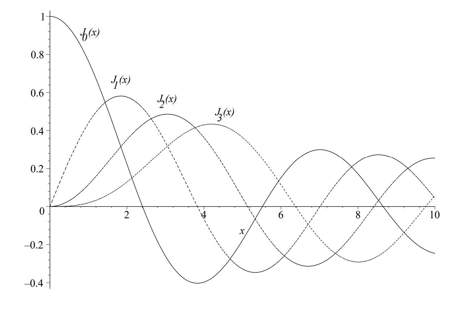
In Figure \(4.3\), we display the first few Bessel functions of the first kind of integer order. Note that these functions can be described as decaying oscillatory functions.

A second linearly independent solution is obtained for \(p\) not an integer as \(J_{-p}(x) .\) However, for \(p\) an integer, the \(\Gamma(n+p+1)\) factor leads to evaluations of the Gamma function at zero, or negative integers, when \(p\) is negative. Thus, the above series is not defined in these cases. Another method for obtaining a second linearly independent solution is through a linear combination of \(J_{p}(x)\) and \(J_{-p}(x)\) as

\[N_{p}(x)=Y_{p}(x)=\dfrac{\cos \pi p J_{p}(x)-J_{-p}(x)}{\sin \pi p} \nonumber \]

These functions are called the Neumann functions, or Bessel functions of the second kind of order \(p\).

Figure \(\PageIndex{2}\): Plots of the Neumann functions \(N_{0}(x), N_{1}(x), N_{2}(x)\), and \(N_{3}(x)\).

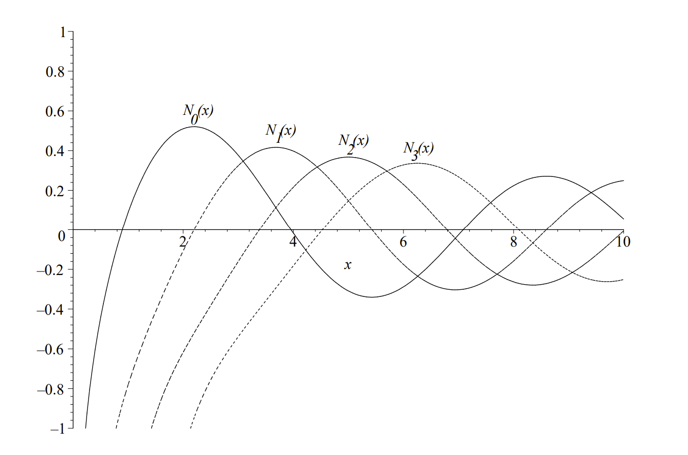
In Figure \(4.4\), we display the first few Bessel functions of the second kind of integer order. Note that these functions are also decaying oscillatory functions. However, they are singular at \(x=0\).

In many applications, one desires bounded solutions at \(x=0\). These functions do not satisfy this boundary condition. For example, one standard problem is to describe the oscillations of a circular drumhead. For this problem one solves the two dimensional wave equation using separation of variables in cylindrical coordinates. The radial equation leads to a Bessel equation. The Bessel function solutions describe the radial part of the solution and one does not expect a singular solution at the center of the drum. The amplitude of the oscillation must remain finite. Thus, only Bessel functions of the first kind can be used.

Bessel functions satisfy a variety of properties, which we will only list at this time for Bessel functions of the first kind. The reader will have the opportunity to prove these for homework.

Derivative Identities. These identities follow directly from the manipulation of the series solution.

\[ \dfrac{d}{d x}\left[x^{p} J_{p}(x)\right] =x^{p} J_{p-1}(x) \nonumber \]

\[\dfrac{d}{d x}\left[x^{-p} J_{p}(x)\right] =-x^{-p} J_{p+1}(x) \nonumber \]

Recursion Formulae. The next identities follow from adding, or subtracting, the derivative identities.

\[J_{p-1}(x)+J_{p+1}(x)=\dfrac{2 p}{x} J_{p}(x) \nonumber \]

\[J_{p-1}(x)-J_{p+1}(x)=2 J_{p}^{\prime}(x) \nonumber \]

Orthogonality. One can recast the Bessel equation into an eigenvalue problem whose solutions form an orthogonal basis of functions on \(L_{x}^{2}(0, a)\). Using Sturm-Liouville Theory, one can show that

\[\int_{0}^{a} x J_{p}\left(j_{p n} \dfrac{x}{a}\right) J_{p}\left(j_{p m} \dfrac{x}{a}\right) d x=\dfrac{a^{2}}{2}\left[J_{p+1}\left(j_{p n}\right)\right]^{2} \delta_{n, m} \nonumber \]

where \(j_{p n}\) is the \(n\)th root of \(J_{p}(x), J_{p}\left(j_{p n}\right)=0, n=1,2, \ldots\) A list of some of these roots is provided in Table \(\PageIndex{1}.\)

Table \(\PageIndex{1}\): The zeros of Bessel Functions, \(J_{m}\left(j_{m n}\right)=0 .\)

\(n\)	\(m=0\)	\(m=1\)	\(m=2\)	\(m=3\)	\(m=4\)	\(m=5\)
1	\(2.405\)	\(3.832\)	\(5.136\)	\(6.380\)	\(7.588\)	\(8.771\)
2	\(5.520\)	\(7.016\)	\(8.417\)	\(9.761\)	\(11.065\)	\(12.339\)
3	\(8.654\)	\(10.173\)	\(11.620\)	\(13.015\)	\(14.373\)	\(15.700\)
4	\(11.792\)	\(13.324\)	\(14.796\)	\(16.223\)	\(17.616\)	\(18.980\)
5	\(14.931\)	\(16.471\)	\(17.960\)	\(19.409\)	\(20.827\)	\(22.218\)
6	\(18.071\)	\(19.616\)	\(21.117\)	\(22.583\)	\(24.019\)	\(25.430\)
7	\(21.212\)	\(22.760\)	\(24.270\)	\(25.748\)	\(27.199\)	\(28.627\)
8	\(24.352\)	\(25.904\)	\(27.421\)	\(28.908\)	\(30.371\)	\(31.812\)
9	\(27.493\)	\(29.047\)	\(30.569\)	\(32.065\)	\(33.537\)	\(34.989\)

Generating Function.

\[e^{x\left(t-\dfrac{1}{t}\right) / 2}=\sum_{n=-\infty}^{\infty} J_{n}(x) t^{n}, \quad x>0, t \neq 0 \nonumber \]

Integral Representation.

\[J_{n}(x)=\dfrac{1}{\pi} \int_{0}^{\pi} \cos (x \sin \theta-n \theta) d \theta, \quad x>0, n \in Z \nonumber \]