5.3: Solution of ODEs Using Laplace Transforms
- Page ID
- 91074

\( \newcommand{\vecs}[1]{\overset { \scriptstyle \rightharpoonup} {\mathbf{#1}} } \)
\( \newcommand{\vecd}[1]{\overset{-\!-\!\rightharpoonup}{\vphantom{a}\smash {#1}}} \)
\( \newcommand{\dsum}{\displaystyle\sum\limits} \)
\( \newcommand{\dint}{\displaystyle\int\limits} \)
\( \newcommand{\dlim}{\displaystyle\lim\limits} \)
\( \newcommand{\id}{\mathrm{id}}\) \( \newcommand{\Span}{\mathrm{span}}\)
( \newcommand{\kernel}{\mathrm{null}\,}\) \( \newcommand{\range}{\mathrm{range}\,}\)
\( \newcommand{\RealPart}{\mathrm{Re}}\) \( \newcommand{\ImaginaryPart}{\mathrm{Im}}\)
\( \newcommand{\Argument}{\mathrm{Arg}}\) \( \newcommand{\norm}[1]{\| #1 \|}\)
\( \newcommand{\inner}[2]{\langle #1, #2 \rangle}\)
\( \newcommand{\Span}{\mathrm{span}}\)
\( \newcommand{\id}{\mathrm{id}}\)
\( \newcommand{\Span}{\mathrm{span}}\)
\( \newcommand{\kernel}{\mathrm{null}\,}\)
\( \newcommand{\range}{\mathrm{range}\,}\)
\( \newcommand{\RealPart}{\mathrm{Re}}\)
\( \newcommand{\ImaginaryPart}{\mathrm{Im}}\)
\( \newcommand{\Argument}{\mathrm{Arg}}\)
\( \newcommand{\norm}[1]{\| #1 \|}\)
\( \newcommand{\inner}[2]{\langle #1, #2 \rangle}\)
\( \newcommand{\Span}{\mathrm{span}}\) \( \newcommand{\AA}{\unicode[.8,0]{x212B}}\)
\( \newcommand{\vectorA}[1]{\vec{#1}} % arrow\)
\( \newcommand{\vectorAt}[1]{\vec{\text{#1}}} % arrow\)
\( \newcommand{\vectorB}[1]{\overset { \scriptstyle \rightharpoonup} {\mathbf{#1}} } \)
\( \newcommand{\vectorC}[1]{\textbf{#1}} \)
\( \newcommand{\vectorD}[1]{\overrightarrow{#1}} \)
\( \newcommand{\vectorDt}[1]{\overrightarrow{\text{#1}}} \)
\( \newcommand{\vectE}[1]{\overset{-\!-\!\rightharpoonup}{\vphantom{a}\smash{\mathbf {#1}}}} \)
\( \newcommand{\vecs}[1]{\overset { \scriptstyle \rightharpoonup} {\mathbf{#1}} } \)
\(\newcommand{\longvect}{\overrightarrow}\)
\( \newcommand{\vecd}[1]{\overset{-\!-\!\rightharpoonup}{\vphantom{a}\smash {#1}}} \)
\(\newcommand{\avec}{\mathbf a}\) \(\newcommand{\bvec}{\mathbf b}\) \(\newcommand{\cvec}{\mathbf c}\) \(\newcommand{\dvec}{\mathbf d}\) \(\newcommand{\dtil}{\widetilde{\mathbf d}}\) \(\newcommand{\evec}{\mathbf e}\) \(\newcommand{\fvec}{\mathbf f}\) \(\newcommand{\nvec}{\mathbf n}\) \(\newcommand{\pvec}{\mathbf p}\) \(\newcommand{\qvec}{\mathbf q}\) \(\newcommand{\svec}{\mathbf s}\) \(\newcommand{\tvec}{\mathbf t}\) \(\newcommand{\uvec}{\mathbf u}\) \(\newcommand{\vvec}{\mathbf v}\) \(\newcommand{\wvec}{\mathbf w}\) \(\newcommand{\xvec}{\mathbf x}\) \(\newcommand{\yvec}{\mathbf y}\) \(\newcommand{\zvec}{\mathbf z}\) \(\newcommand{\rvec}{\mathbf r}\) \(\newcommand{\mvec}{\mathbf m}\) \(\newcommand{\zerovec}{\mathbf 0}\) \(\newcommand{\onevec}{\mathbf 1}\) \(\newcommand{\real}{\mathbb R}\) \(\newcommand{\twovec}[2]{\left[\begin{array}{r}#1 \\ #2 \end{array}\right]}\) \(\newcommand{\ctwovec}[2]{\left[\begin{array}{c}#1 \\ #2 \end{array}\right]}\) \(\newcommand{\threevec}[3]{\left[\begin{array}{r}#1 \\ #2 \\ #3 \end{array}\right]}\) \(\newcommand{\cthreevec}[3]{\left[\begin{array}{c}#1 \\ #2 \\ #3 \end{array}\right]}\) \(\newcommand{\fourvec}[4]{\left[\begin{array}{r}#1 \\ #2 \\ #3 \\ #4 \end{array}\right]}\) \(\newcommand{\cfourvec}[4]{\left[\begin{array}{c}#1 \\ #2 \\ #3 \\ #4 \end{array}\right]}\) \(\newcommand{\fivevec}[5]{\left[\begin{array}{r}#1 \\ #2 \\ #3 \\ #4 \\ #5 \\ \end{array}\right]}\) \(\newcommand{\cfivevec}[5]{\left[\begin{array}{c}#1 \\ #2 \\ #3 \\ #4 \\ #5 \\ \end{array}\right]}\) \(\newcommand{\mattwo}[4]{\left[\begin{array}{rr}#1 \amp #2 \\ #3 \amp #4 \\ \end{array}\right]}\) \(\newcommand{\laspan}[1]{\text{Span}\{#1\}}\) \(\newcommand{\bcal}{\cal B}\) \(\newcommand{\ccal}{\cal C}\) \(\newcommand{\scal}{\cal S}\) \(\newcommand{\wcal}{\cal W}\) \(\newcommand{\ecal}{\cal E}\) \(\newcommand{\coords}[2]{\left\{#1\right\}_{#2}}\) \(\newcommand{\gray}[1]{\color{gray}{#1}}\) \(\newcommand{\lgray}[1]{\color{lightgray}{#1}}\) \(\newcommand{\rank}{\operatorname{rank}}\) \(\newcommand{\row}{\text{Row}}\) \(\newcommand{\col}{\text{Col}}\) \(\renewcommand{\row}{\text{Row}}\) \(\newcommand{\nul}{\text{Nul}}\) \(\newcommand{\var}{\text{Var}}\) \(\newcommand{\corr}{\text{corr}}\) \(\newcommand{\len}[1]{\left|#1\right|}\) \(\newcommand{\bbar}{\overline{\bvec}}\) \(\newcommand{\bhat}{\widehat{\bvec}}\) \(\newcommand{\bperp}{\bvec^\perp}\) \(\newcommand{\xhat}{\widehat{\xvec}}\) \(\newcommand{\vhat}{\widehat{\vvec}}\) \(\newcommand{\uhat}{\widehat{\uvec}}\) \(\newcommand{\what}{\widehat{\wvec}}\) \(\newcommand{\Sighat}{\widehat{\Sigma}}\) \(\newcommand{\lt}{<}\) \(\newcommand{\gt}{>}\) \(\newcommand{\amp}{&}\) \(\definecolor{fillinmathshade}{gray}{0.9}\)ONE OF THE TYPICAL APPLICATIONS OF LAPLACE TRANSFORMS is the solution of nonhomogeneous linear constant coefficient differential equations. In the following examples we will show how this works.
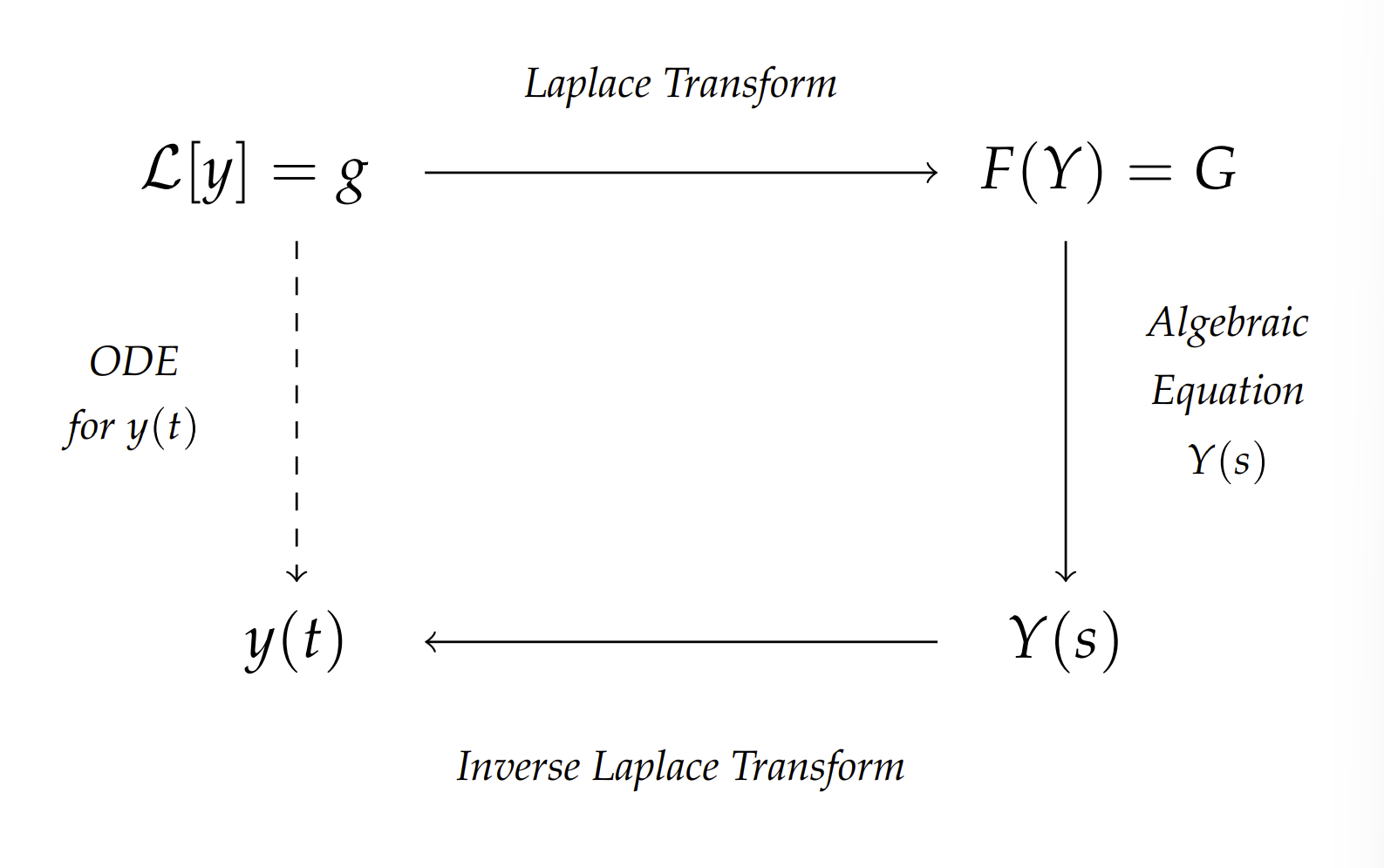
The general idea is that one transforms the equation for an unknown function \(y(t)\) into an algebraic equation for its transform, \(Y(t)\). Typically, the algebraic equation is easy to solve for \(Y(s)\) as a function of \(s\). Then, one transforms back into \(t\)-space using Laplace transform tables and the properties of Laplace transforms. The scheme is shown in Figure \(5 \cdot 2 \).
Solve the initial value problem \(y^{\prime}+3 y=e^{2 t}, y(0)=1\).
The first step is to perform a Laplace transform of the initial value problem. The transform of the left side of the equation is
\[\mathcal{L}\left[y^{\prime}+3 y\right]=s Y-y(0)+3 Y=(s+3) Y-1 \nonumber \]
Transforming the right-hand side, we have
\[\mathcal{L}\left[e^{2 t}\right]=\dfrac{1}{s-2} \nonumber \]
Combining these two results, we obtain
\[(s+3) Y-1=\dfrac{1}{s-2}\nonumber \]
The next step is to solve for \(Y(s)\) :
\[Y(s)=\dfrac{1}{s+3}+\dfrac{1}{(s-2)(s+3)}\nonumber \]
Now we need to find the inverse Laplace transform. Namely, we need to figure out what function has a Laplace transform of the above form. We will use the tables of Laplace transform pairs. Later we will show that there are other methods for carrying out the Laplace transform inversion.
The inverse transform of the first term is \(e^{-3 t}\). However, we have not seen anything that looks like the second form in the table of transforms that we have compiled, but we can rewrite the second term using a partial fraction decomposition. Let’s recall how to do this.
The goal is to find constants \(A\) and \(B\) such that
\[\dfrac{1}{(s-2)(s+3)}=\dfrac{A}{s-2}+\dfrac{B}{s+3} \nonumber \]
We picked this form because we know that recombining the two terms into one term will have the same denominator. We just need to make sure the numerators agree afterward. So, adding the two terms, we have
\[\dfrac{1}{(s-2)(s+3)}=\dfrac{A(s+3)+B(s-2)}{(s-2)(s+3)} \nonumber \]
Equating numerators,
\[1=A(s+3)+B(s-2)\nonumber \]
There are several ways to proceed at this point.
a. Method 1.
We can rewrite the equation by gathering terms with common powers of \(s\), we have
\[(A+B) s+3 A-2 B=1 \nonumber \]
The only way that this can be true for all \(s\) is that the coefficients of the different powers of \(s\) agree on both sides. This leads to two equations for \(A\) and \(B\) :
\[ \begin{array}{r} A+B=0 \\[4pt] 3 A-2 B=1 \end{array}\label{5.15} \]
The first equation gives \(A=-B\), so the second equation becomes \(-5 B=1 \). The solution is then \(A=-B=\dfrac{1}{5} \).
b. Method 2 .
Since the equation \(\dfrac{1}{(s-2)(s+3)}=\dfrac{A}{s-2}+\dfrac{B}{s+3}\) is true for all \(s\), we can pick specific values. For \(s=2\), we find \(1=5 A\), or \(A=\dfrac{1}{5} \). For \(s=-3\), we find \(1=-5 B\), or \(B=-\dfrac{1}{5} \). Thus, we obtain the same result as Method 1, but much quicker.
This is an example of carrying out a partial fraction decomposition.
c. Method 3.
We could just inspect the original partial fraction problem. Since the numerator has no \(s\) terms, we might guess the form
\[\dfrac{1}{(s-2)(s+3)}=\dfrac{1}{s-2}-\dfrac{1}{s+3} \nonumber \]
But, recombining the terms on the right-hand side, we see that
\[\dfrac{1}{s-2}-\dfrac{1}{s+3}=\dfrac{5}{(s-2)(s+3)}\nonumber \]
Since we were off by 5, we divide the partial fractions by 5 to obtain
\[\dfrac{1}{(s-2)(s+3)}=\dfrac{1}{5}\left[\dfrac{1}{s-2}-\dfrac{1}{s+3}\right]\nonumber \]
which once again gives the desired form.
Returning to the problem, we have found that
\[Y(s)=\dfrac{1}{s+3}+\dfrac{1}{5}\left(\dfrac{1}{s-2}-\dfrac{1}{s+3}\right)\nonumber \]
We can now see that the function with this Laplace transform is given by
\[y(t)=\mathcal{L}^{-1}\left[\dfrac{1}{s+3}+\dfrac{1}{5}\left(\dfrac{1}{s-2}-\dfrac{1}{s+3}\right)\right]=e^{-3 t}+\dfrac{1}{5}\left(e^{2 t}-e^{-3 t}\right) \nonumber \]
works. Simplifying, we have the solution of the initial value problem
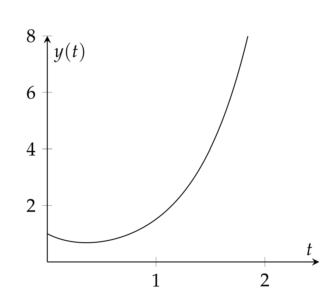
\[y(t)=\dfrac{1}{5} e^{2 t}+\dfrac{4}{5} e^{-3 t}\nonumber \]
We can verify that we have solved the initial value problem.
\[y^{\prime}+3 y=\dfrac{2}{5} e^{2 t}-\dfrac{12}{5} e^{-3 t}+3\left(\dfrac{1}{5} e^{2 t}+\dfrac{4}{5} e^{-3 t}\right)=e^{2 t}\nonumber \]
and \(y(0)=\dfrac{1}{5}+\dfrac{4}{5}=1\).
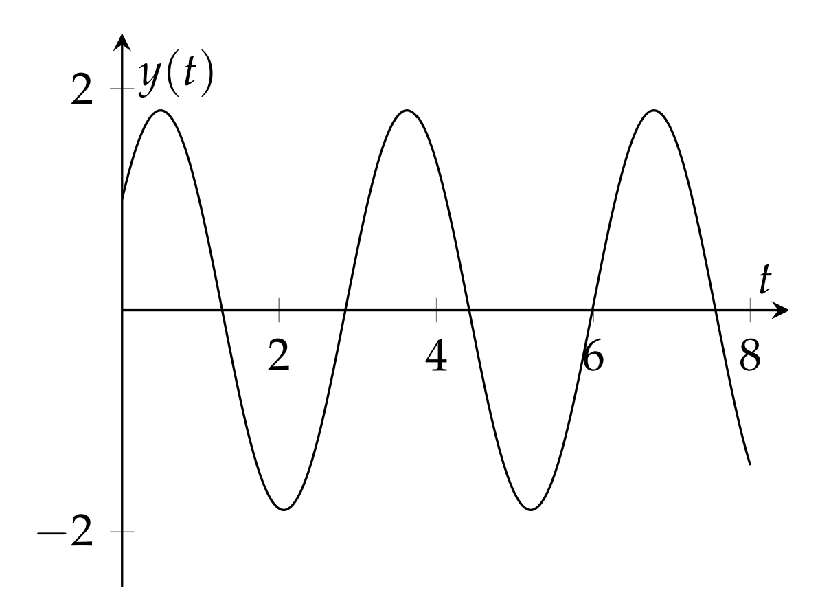
Solve the initial value problem \(y^{\prime \prime}+4 y=0, y(0)=1\), \(y^{\prime}(0)=3 \).
We can probably solve this without Laplace transforms, but it is a simple exercise. Transforming the equation, we have
\[\begin{aligned} 0 &=s^{2} Y-s y(0)-y^{\prime}(0)+4 Y \\[4pt] &=\left(s^{2}+4\right) Y-s-3 \end{aligned}\label{5.16} \]
Solving for \(Y\), we have
\[Y(s)=\dfrac{s+3}{s^{2}+4}\nonumber \]
We now ask if we recognize the transform pair needed. The denominator looks like the type needed for the transform of a sine or cosine. We just need to play with the numerator. Splitting the expression into two terms, we have
\[Y(s)=\dfrac{s}{s^{2}+4}+\dfrac{3}{s^{2}+4}\nonumber \]
The first term is now recognizable as the transform of \(\cos 2 t\). The second term is not the transform of \(\sin 2 t\). It would be if the numerator were a 2 . This can be corrected by multiplying and dividing by 2 :
\[\dfrac{3}{s^{2}+4}=\dfrac{3}{2}\left(\dfrac{2}{s^{2}+4}\right)\nonumber \]
The solution is then found as
\[y(t)=\mathcal{L}^{-1}\left[\dfrac{s}{s^{2}+4}+\dfrac{3}{2}\left(\dfrac{2}{s^{2}+4}\right)\right]=\cos 2 t+\dfrac{3}{2} \sin 2 t \nonumber \]
The reader can verify that this is the solution of the initial value problem and is shown in Figure \(\PageIndex{2}\).