5.4: Step and Impulse Functions


- Last updated
- May 24, 2024
- Save as PDF

( \newcommand{\kernel}{\mathrm{null}\,}\)
Heaviside Step Function
OFTEN, THE INITIAL VALUE PROBLEMS THAT ONE FACES in differential equations courses can be solved using either the Method of Undetermined Coefficients or the Method of Variation of Parameters. However, using the latter can be messy and involves some skill with integration. Many circuit designs can be modeled with systems of differential equations using Kirchoff’s Rules. Such systems can get fairly complicated. However, Laplace transforms can be used to solve such systems, and electrical engineers have long used such methods in circuit analysis.
In this section we add a couple more transform pairs and transform properties that are useful in accounting for things like turning on a driving force, using periodic functions like a square wave, or introducing impulse forces.
We first recall the Heaviside step function, given by
H(t)={0,t<01,t>0
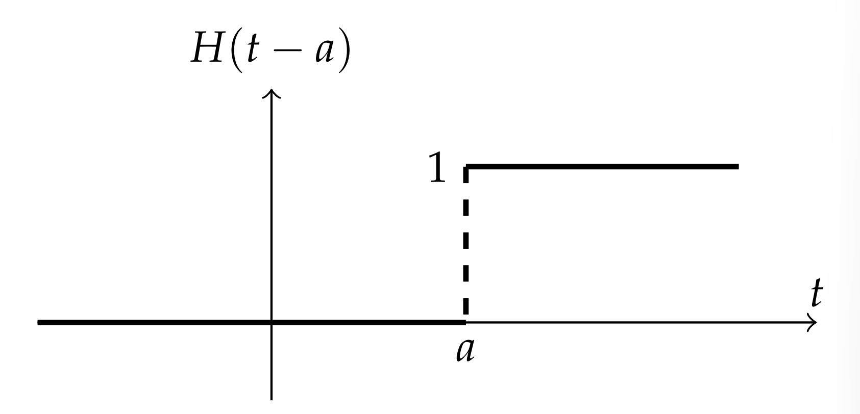
. A more general version of the step function is the horizontally shifted step function, H(t−a). This function is shown in Figure 5⋅5. The Laplace transform of this function is found for a>0 as
L[H(t−a)]=∫∞0H(t−a)e−stdt=∫∞ae−stdt=e−sts|∞a=e−ass
The Laplace transform has two Shift Theorems involving the multiplication of the function, f(t), or its transform, F(s), by exponentials. The First and Second Shift Properties Theorems are given by
L[eatf(t)]=F(s−a)
L[f(t−a)H(t−a)]=e−asF(s).
(The Shift Theorems). We prove the First Shift Theorem and leave the other proof as an exercise for the reader. Namely,
L[eatf(t)]=∫∞0eatf(t)e−stdt=∫∞0f(t)e−(s−a)tdt=F(s−a)
Compute the Laplace transform of e−atsinωt.
This function arises as the solution of the underdamped harmonic oscillator. We first note that the exponential multiplies a sine function. The First Shift Theorem tells us that we first need the transform of the sine function. So, for f(t)=sinωt, we have
F(s)=ωs2+ω2
Using this transform, we can obtain the solution to this problem as
L[e−atsinωt]=F(s+a)=ω(s+a)2+ω2
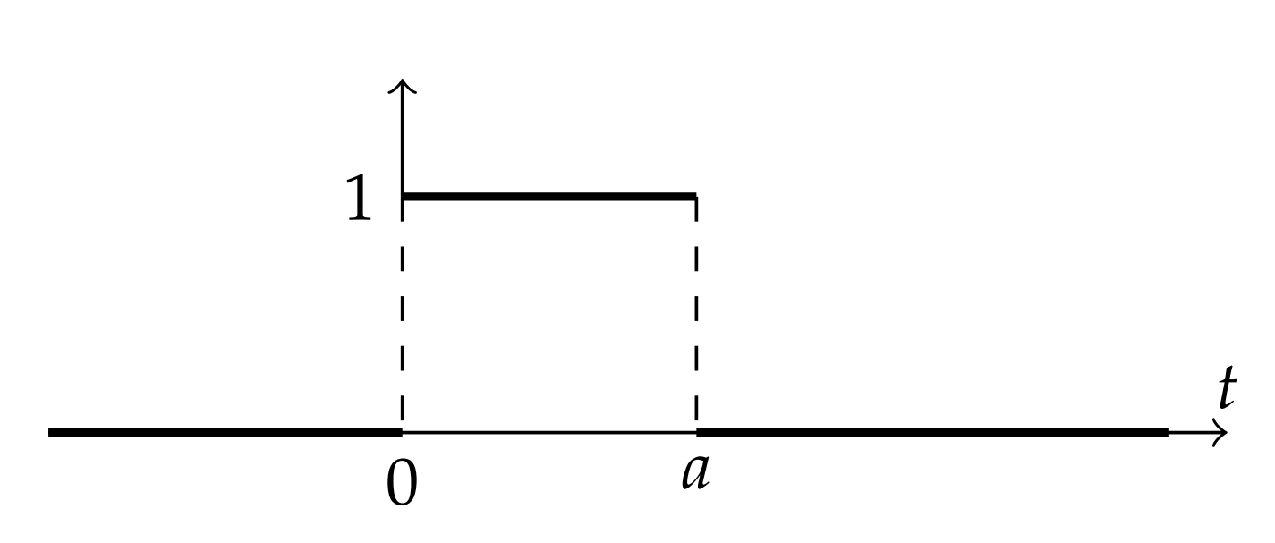
More interesting examples can be found using piecewise defined functions. First we consider the function H(t)−H(t−a). For t<0, both terms are zero. In the interval [0,a], the function H(t)=1 and H(t−a)=0. Therefore, H(t)−H(t−a)=1 for t∈[0,a]. Finally, for t>a, both functions are one and therefore the difference is zero. The graph of H(t)−H(t−a) is shown in Figure 5.4.2.
We now consider the piecewise defined function:
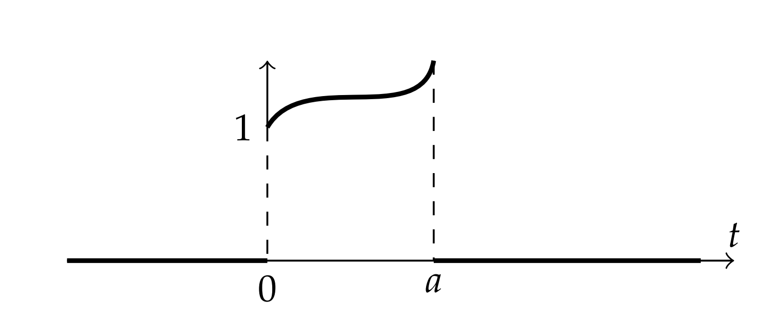
g(t)={f(t),0≤t≤a0,t<0,t>a
This function can be rewritten in terms of step functions. We only need to multiply f(t) by the above box function,
g(t)=f(t)[H(t)−H(t−a)].
We depict this in Figure 5.4.3.
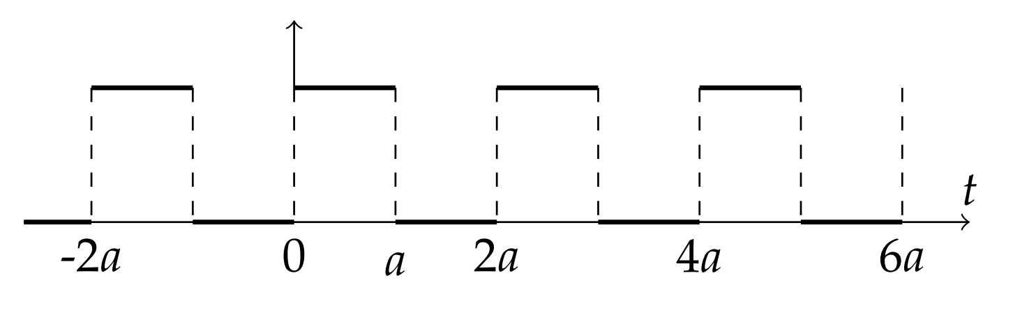
Even more complicated functions can be written in terms of step functions. We only need to look at sums of functions of the form f(t)[H(t−a)−H(t−b)] for b>a. This is similar to a box function. It is nonzero between a and b and has height f(t). We show as an example the square wave function in Figure 5.4.4. It can be represented as a sum of an infinite number of boxes,
f(t)=∞∑n=−∞[H(t−2na)−H(t−(2n+1)a)]
for a>0
Find the Laplace Transform of a square wave "turned on′′ at t=0.
We let
f(t)=∞∑n=0[H(t−2na)−H(t−(2n+1)a)],a>0
Using the properties of the Heaviside function, we have
L[f(t)]=∞∑n=0[L[H(t−2na)]−L[H(t−(2n+1)a)]]=∞∑n=0[e−2nass−e−(2n+1)ass]=1−e−ass∞∑n=0(e−2as)n=1−e−ass(11−e−2as)=1−e−ass(1−e−2as)=1s(1+e−as)
Note that the third line in the derivation is a geometric series. We summed this series to get the answer in a compact form since e−2as< 1.
Periodic Functions∗
The previous example provides us with a causal function (f(t)=0 for t<0.) which is periodic with period a. Such periodic functions can be teated in a simpler fashion. We will now show that
(Laplace transform of periodic functions).
If f(t) is periodic with period T and piecewise continuous on [0,T], then
F(s)=11−e−sT∫T0f(t)e−stdt
- Proof.
-
F(s)=∫∞0f(t)e−stdt=∫T0f(t)e−stdt+∫∞Tf(t)e−stdt=∫T0f(t)e−stdt+∫∞Tf(t−T)e−stdt=∫T0f(t)e−stdt+e−sT∫∞0f(τ)e−sτdτ=∫T0f(t)e−stdt+e−sTF(s)
Solving for F(s), one obtains the desired result.
Use the periodicity of
f(t)=∞∑n=0[H(t−2na)−H(t−(2n+1)a)],a>0
to obtain the Laplace transform.
We note that f(t) has period T=2a. By Theorem 5.1, we have
F(s)=∫∞0f(t)e−stdt=11−e−2as∫2a0[H(t)−H(t−a)]e−stdt=11−e−2as[∫2a0e−stdt−∫2aae−stdt]=11−e−2as[e−st−s|2a0−e−st−s|2aa]=1s(1−e−2as)[1−e−2as+e−2as−e−as]=1−e−ass(1−e−2as)=1s(1+e−as)
This is the same result that was obtained in the previous example.
P. A. M. Dirac (1902−1984) introduced the δ function in his book, The Principles of Quantum Mechanics, 4 th Ed., Ox− ford University Press, 1958 , originally published in 1930 , as part of his orthogonality statement for a basis of functions in a Hilbert space, ⟨ξ′∣ξ′′⟩= cδ(ξ′−ζ′′) in the same way we introduced discrete orthogonality using the Kronecker delta. Historically, a number of mathematicians sought to understand the Diract delta function, culminating in Laurent Schwartz’s (1915-2002) theory of distributions in 1945 .
Dirac Delta Function
ANOTHER USEFUL CONCEPT IS THE IMPULSE FUNCTION. If wE want to apply an impulse function, we can use the Dirac delta function δ(x). This is an example of what is known as a generalized function, or a distribution. Dirac had introduced this function in the 1930 s in his study of quantum mechanics as a useful tool. It was later studied in a general theory of distributions and found to be more than a simple tool used by physicists. The Dirac delta function, as any distribution, only makes sense under an integral. Here will will introduce the Dirac delta function through its main properties. The delta function satisfies two main properties:
- δ(x)=0 for x≠0.
- ∫∞−∞δ(x)dx=1.
Integration over more general intervals gives
∫baδ(x)dx={1,0∈[a,b]0,0∉[a,b]
Another important property is the sifting property:
∫∞−∞δ(x−a)f(x)dx=f(a)
This can be seen by noting that the delta function is zero everywhere except at x=a. Therefore, the integrand is zero everywhere and the only contribution from f(x) will be from x=a. So, we can replace f(x) with f(a) under the integral. Since f(a) is a constant, we have that
∫∞−∞δ(x−a)f(x)dx=∫∞−∞δ(x−a)f(a)dx=f(a)∫∞−∞δ(x−a)dx=f(a)
Evaluate: ∫∞−∞δ(x+3)x3dx
This is a simple use of the sifting property:
∫∞−∞δ(x+3)x3dx=(−3)3=−27
Another property results from using a scaled argument, ax. In this case, we show that
δ(ax)=|a|−1δ(x)
usual, this only has meaning under an integral sign. So, we place δ(ax) inside an integral and make a substitution y=ax :
∫∞−∞δ(ax)dx=limL→∞∫L−Lδ(ax)dx=limL→∞1a∫aL−aLδ(y)dy
If a>0 then
∫∞−∞δ(ax)dx=1a∫∞−∞δ(y)dy
However, if a<0 then
∫∞−∞δ(ax)dx=1a∫−∞∞δ(y)dy=−1a∫∞−∞δ(y)dy
The overall difference in a multiplicative minus sign can be absorbed into one expression by changing the factor 1/a to 1/|a|. Thus,
∫∞−∞δ(ax)dx=1|a|∫∞−∞δ(y)dy
Properties of the Dirac delta function:
∫∞−∞δ(x−a)f(x)dx=f(a).∫∞−∞δ(ax)dx=1|a|∫∞−∞δ(y)dy.
Evaluate ∫∞−∞(5x+1)δ(4(x−2))dx
This is a straightforward integration:
∫∞−∞(5x+1)δ(4(x−2))dx=14∫∞−∞(5x+1)δ(x−2)dx=114
The first step is to write δ(4(x−2))=14δ(x−2). Then, the final evaluation is given by
14∫∞−∞(5x+1)δ(x−2)dx=14(5(2)+1)=114
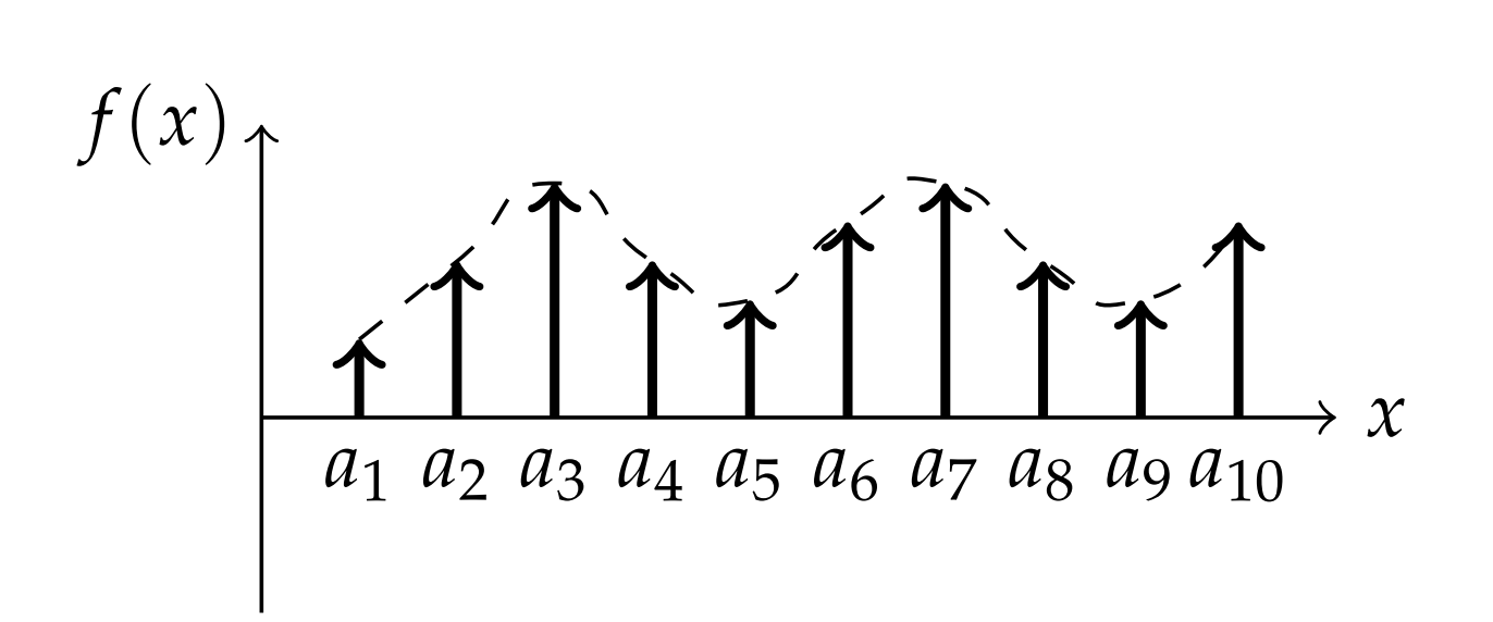
The Dirac delta function can be used to represent a unit impulse. Summing over a number of impulses, or point sources, we can describe a general function as shown in Figure 5.9. The sum of impulses located at points ai, i=1,…,n, with strengths f(ai) would be given by
f(x)=n∑i=1f(ai)δ(x−ai)
A continuous sum could be written as
f(x)=∫∞−∞f(ξ)δ(x−ξ)dξ
This is simply an application of the sifting property of the delta function.
We will investigate a case when one would use a single impulse. While a mass on a spring is undergoing simple harmonic motion, we hit it for an instant at time t=a. In such a case, we could represent the force as a multiple of \(\delta(t − a) \\[4pt]).
One would then need the Laplace transform of the delta function to solve the associated initial value problem. Inserting the delta function into the Laplace transform, we find that for a>0,
L[δ(t−a)]=∫∞0δ(t−a)e−stdt=∫∞−∞δ(t−a)e−stdt=e−as
Solve the initial value problem y′′+4π2y=δ(t−2),
This initial value problem models a spring oscillation with an impulse force. Without the forcing term, given by the delta function, this spring is initially at rest and not stretched. The delta function models a unit impulse at t=2. Of course, we anticipate that at this time the spring will begin to oscillate. We will solve this problem using Laplace y(0)=y′(0)=0. transforms. First, we transform the differential equation:
s2Y−sy(0)−y′(0)+4π2Y=e−2s
Inserting the initial conditions, we have
(s2+4π2)Y=e−2s
Solving for Y(s), we obtain
Y(s)=e−2ss2+4π2
We now seek the function for which this is the Laplace transform. The form of this function is an exponential times some Laplace transform, F(s). Thus, we need the Second Shift Theorem since the solution is of the form Y(s)=e−2sF(s) for
F(s)=1s2+4π2.
We need to find the corresponding f(t) of the Laplace transform pair. The denominator in F(s) suggests a sine or cosine. Since the numerator is constant, we pick sine. From the tables of transforms, we have
L[sin2πt]=2πs2+4π2
So, we write
F(s)=12π2πs2+4π2
This gives f(t)=(2π)−1sin2πt.
We now apply the Second Shift Theorem, L[f(t−a)H(t−a)]= e−asF(s), or
y(t)=L−1[e−2sF(s)]=H(t−2)f(t−2)=12πH(t−2)sin2π(t−2)
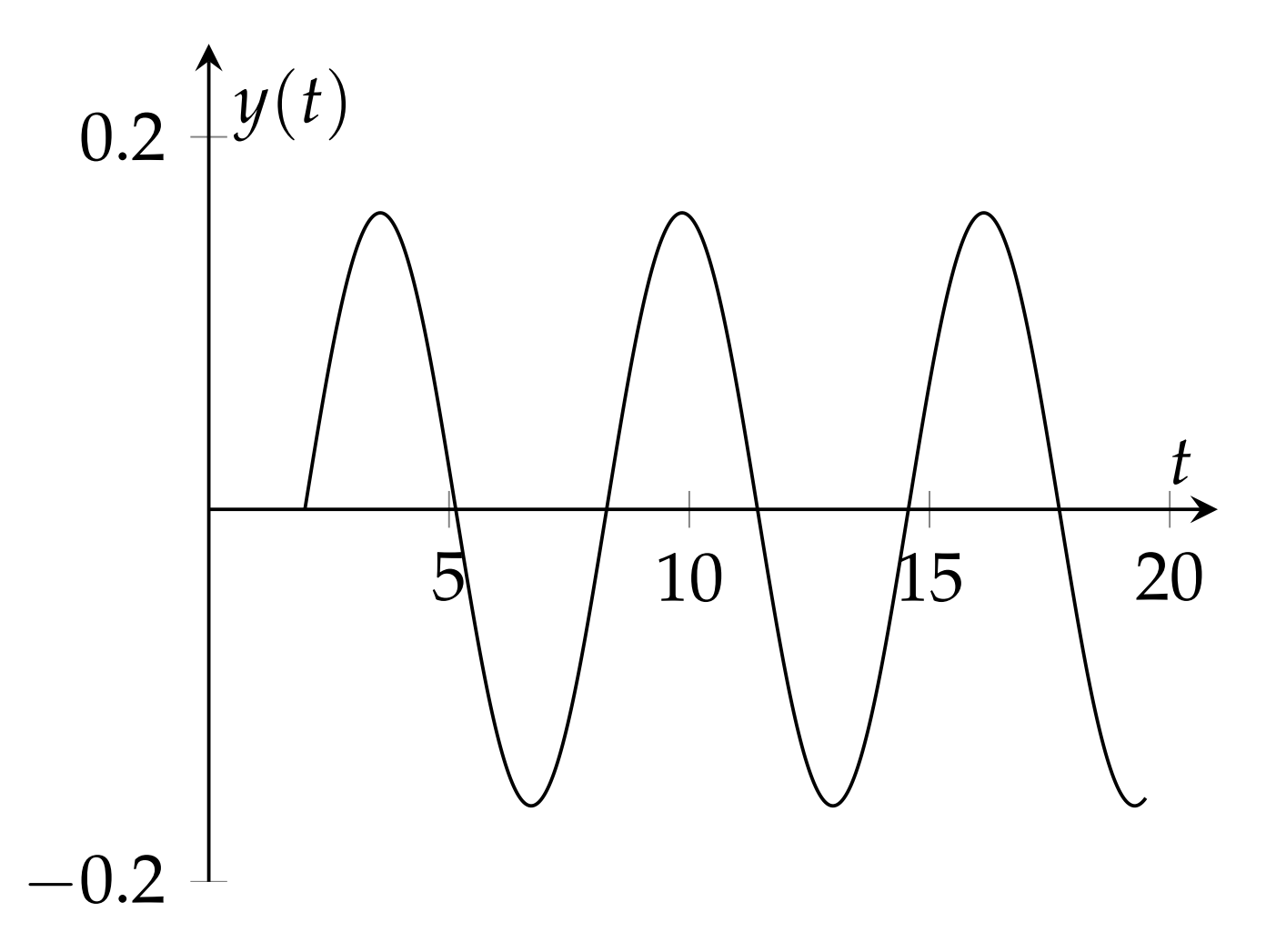
This solution tells us that the mass is at rest until t=2 and then ample 5.14 in which a spring at rest exbegins to oscillate at its natural frequency. A plot of this solution is periences an impulse force at t=2. shown in Figure 5.4.6
Solve the initial value problem
y′′+y=f(t),y(0)=0,y′(0)=0
where
f(t)={cosπt,0≤t≤20, otherwise
We need the Laplace transform of f(t). This function can be written in terms of a Heaviside function, f(t)=cosπtH(t−2). In order to apply the Second Shift Theorem, we need a shifted version of the cosine function. We find the shifted version by noting that cosπ(t−2)=cosπt. Thus, we have
f(t)=cosπt[H(t)−H(t−2)]=cosπt−cosπ(t−2)H(t−2),t≥0
The Laplace transform of this driving term is
F(s)=(1−e−2s)L[cosπt]=(1−e−2s)ss2+π2
Now we can proceed to solve the initial value problem. The Laplace transform of the initial value problem yields
(s2+1)Y(s)=(1−e−2s)ss2+π2
Therefore,
Y(s)=(1−e−2s)s(s2+π2)(s2+1)
We can retrieve the solution to the initial value problem using the Second Shift Theorem. The solution is of the form Y(s)=(1− e−2s)G(s) for
G(s)=s(s2+π2)(s2+1)
Then, the final solution takes the form
y(t)=g(t)−g(t−2)H(t−2)
We only need to find g(t) in order to finish the problem. This is easily done using the partial fraction decomposition
G(s)=s(s2+π2)(s2+1)=1π2−1[ss2+1−ss2+π2]
Then,
g(t)=L−1[s(s2+π2)(s2+1)]=1π2−1(cost−cosπt)
The final solution is then given by
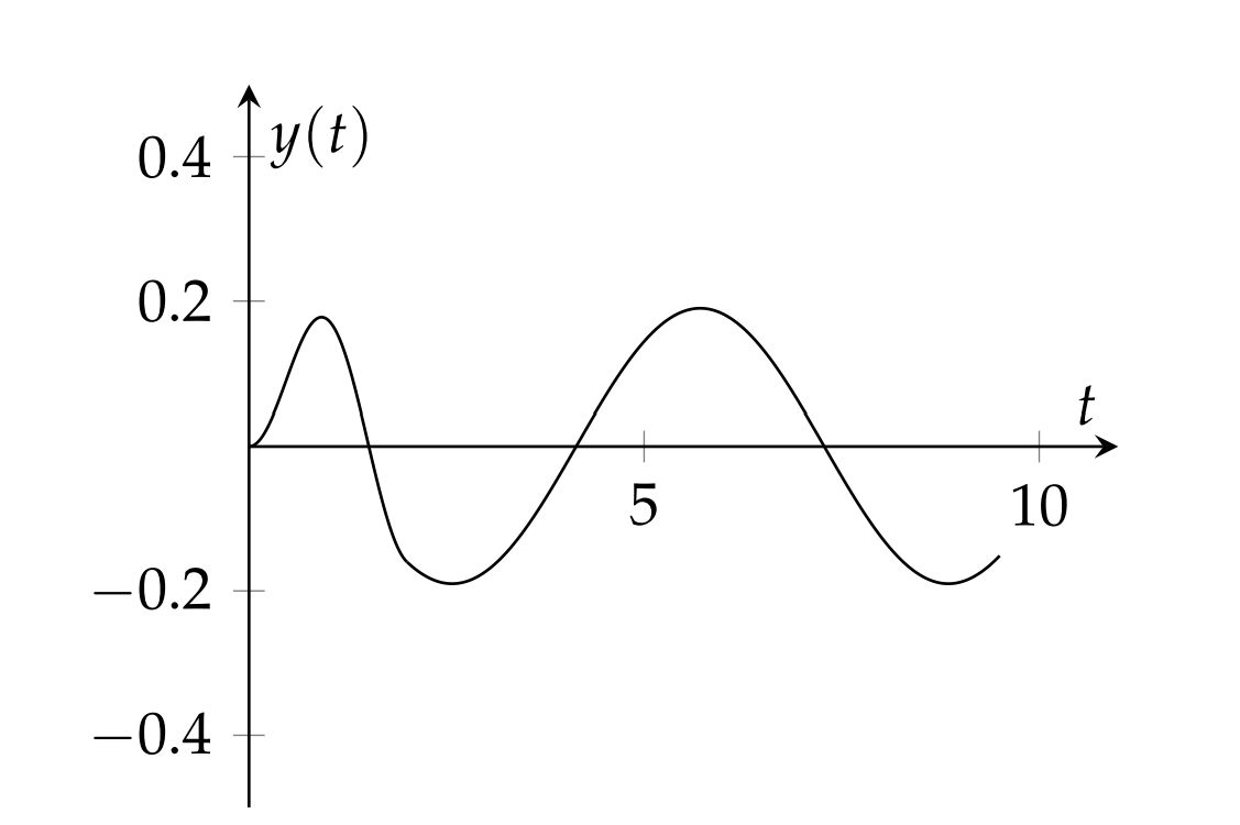
y(t)=1π2−1[cost−cosπt−H(t−2)(cos(t−2)−cosπt)]
A plot of this solution is shown in Figure 5.4.7.