
6.2.1: Mass-Spring Systems
- Page ID
- 107198

THE FIRST EXAMPLES THAT WE HAD SEEN involved masses on springs. Recall that for a simple mass on a spring we studied simple harmonic motion, which is governed by the equation
\[m \ddot{x}+k x=0\nonumber \]
This second order equation can be written as two first order equations
\[\begin{array}{r} \dot{x}=y \\ \dot{y}=-\dfrac{k}{m} x \end{array} \nonumber \]
or
\[\begin{array}{r} \dot{x}=y \\ \dot{y}=-\omega^{2} x \end{array} \nonumber \]
where \(\omega^{2}=\dfrac{k}{m}\). The coefficient matrix for this system is
\[A=\left(\begin{array}{cc} 0 & 1 \\ -\omega^{2} & 0 \end{array}\right) \nonumber \]
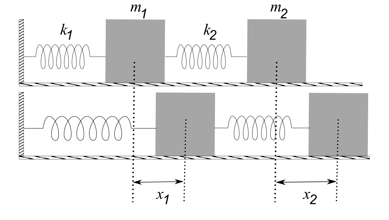
We also looked at the system of two masses and two springs as shown in Figure \(6.20\). The equations governing the motion of the masses is
\[ \begin{aligned} &m_{1} \ddot{x}_{1}=-k_{1} x_{1}+k_{2}\left(x_{2}-x_{1}\right) \\ &m_{2} \ddot{x}_{2}=-k_{2}\left(x_{2}-x_{1}\right) \end{aligned} \label{6.40} \]
We can rewrite this system as four first order equations
\[ \begin{aligned} \dot{x}_{1} &=x_{3} \\ \dot{x}_{2} &=x_{4} \\ \dot{x}_{3} &=-\dfrac{k_{1}}{m_{1}} x_{1}+\dfrac{k_{2}}{m_{1}}\left(x_{2}-x_{1}\right) \\ \dot{x}_{4} &=-\dfrac{k_{2}}{m_{2}}\left(x_{2}-x_{1}\right) \end{aligned} \label{6.41} \]
The coefficient matrix for this system is
\[A=\left(\begin{array}{cccc}
0 & 0 & 1 & 0 \\
0 & 0 & 0 & 1 \\
-\dfrac{k_{1}+k_{2}}{m_{1}} & \dfrac{k_{2}}{m_{1}} & 0 & 0 \\
\dfrac{k_{2}}{m_{2}} & -\dfrac{k_{2}}{m_{2}} & 0 & 0
\end{array}\right) \nonumber \]
We can study this system for specific values of the constants using the methods covered in the last sections.
Writing the spring-block system as a second order vector system.
\[\left(\begin{array}{cc}
m_{1} & 0 \\
0 & m_{2}
\end{array}\right)\left(\begin{array}{c}
\ddot{x}_{1} \\
\ddot{x}_{2}
\end{array}\right)=\left(\begin{array}{cc}
-\left(k_{1}+k_{2}\right) & k_{2} \\
k_{2} & -k_{2}
\end{array}\right)\left(\begin{array}{l}
x_{1} \\
x_{2}
\end{array}\right). \nonumber \]
This system can then be written compactly as
\[ M \ddot{\mathbf{x}}=-K \mathbf{x}, \nonumber \]
where
\[M=\left(\begin{array}{cc} m_{1} & 0 \\ 0 & m_{2} \end{array}\right), \quad K=\left(\begin{array}{cc} k_{1}+k_{2} & -k_{2} \\ -k_{2} & k_{2} \end{array}\right) \nonumber \]
This system can be solved by guessing a form for the solution. We could guess
\[\mathbf{x}=\mathbf{a} e^{i \omega t} \nonumber \]
Or
\[\mathbf{x}=\left(\begin{array}{l} a_{1} \cos \left(\omega t-\delta_{1}\right) \\ a_{2} \cos \left(\omega t-\delta_{2}\right) \end{array}\right)\nonumber \]
where \(\delta_{i}\) are phase shifts determined from initial conditions.
Inserting \(\mathbf{x}=\mathbf{a} e^{i \omega t}\) into the system gives
\[\left(K-\omega^{2} M\right) \mathbf{a}=\mathbf{0} \nonumber \]
This is a homogeneous system. It is a generalized eigenvalue problem for eigenvalues \(\omega^{2}\) and eigenvectors a. We solve this in a similar way to the standard matrix eigenvalue problems. The eigenvalue equation is found as
\[\operatorname{det}\left(K-\omega^{2} M\right)=0\nonumber \]
Once the eigenvalues are found, then one determines the eigenvectors and constructs the solution.
Let \(m_{1}=m_{2}=m\) and \(k_{1}=k_{2}=k\). Then, we have to solve the system
\[\omega^{2}\left(\begin{array}{cc} m & 0 \\ 0 & m \end{array}\right)\left(\begin{array}{l} a_{1} \\ a_{2} \end{array}\right)=\left(\begin{array}{cc} 2 k & -k \\ -k & k \end{array}\right)\left(\begin{array}{l} a_{1} \\ a_{2} \end{array}\right)\nonumber \]
The eigenvalue equation is given by
\[ \begin{aligned} 0 &=\left|\begin{array}{cc} 2 k-m \omega^{2} & -k \\ -k & k-m \omega^{2} \end{array}\right| \\ &=\left(2 k-m \omega^{2}\right)\left(k-m \omega^{2}\right)-k^{2} \\ &=m^{2} \omega^{4}-3 k m \omega^{2}+k^{2} \end{aligned} \label{6.44} \]
Solving this quadratic equation for \(\omega^{2}\), we have
\[\omega^{2}=\dfrac{3 \pm 1}{2} \dfrac{k}{m}\nonumber \]
For positive values of \(\omega\), one can show that
\[\omega=\dfrac{1}{2}(\pm 1+\sqrt{5}) \sqrt{\dfrac{k}{m}}\nonumber \]
The eigenvectors can be found for each eigenvalue by solving the homogeneous system
\[\left(\begin{array}{cc} 2 k-m \omega^{2} & -k \\ -k & k-m \omega^{2} \end{array}\right)\left(\begin{array}{c} a_{1} \\ a_{2} \end{array}\right)=0\nonumber \]
The eigenvectors are given by
\[\mathbf{a}_{1}=\left(\begin{array}{c} -\dfrac{\sqrt{5}+1}{2} \\ 1 \end{array}\right), \quad \mathbf{a}_{2}=\left(\begin{array}{c} \dfrac{\sqrt{5}-1}{2} \\ 1 \end{array}\right)\nonumber \]
We are now ready to construct the real solutions to the problem. Similar to solving two first order systems with complex roots, we take the real and imaginary parts and take a linear combination of the solutions. In this problem there are four terms, giving the solution in the form
\[\mathbf{x}(t)=c_{1} \mathbf{a}_{1} \cos \omega_{1} t+c_{2} \mathbf{a}_{1} \sin \omega_{1} t+c_{3} \mathbf{a}_{2} \cos \omega_{2} t+c_{4} \mathbf{a}_{2} \sin \omega_{2} t\nonumber \]
where the \(\omega^{\prime}\) s are the eigenvalues and the a’s are the corresponding eigenvectors. The constants are determined from the initial conditions, \(\mathbf{x}(0)=\mathbf{x}_{0}\) and \(\dot{\mathbf{x}}(0)=\mathbf{v}_{0} .\)