6.2.2: Circuits

Last updated
Save as PDF

Page ID: 107199

\( \newcommand{\vecs}[1]{\overset { \scriptstyle \rightharpoonup} {\mathbf{#1}} } \) \( \newcommand{\vecd}[1]{\overset{-\!-\!\rightharpoonup}{\vphantom{a}\smash {#1}}} \)\(\newcommand{\id}{\mathrm{id}}\) \( \newcommand{\Span}{\mathrm{span}}\) \( \newcommand{\kernel}{\mathrm{null}\,}\) \( \newcommand{\range}{\mathrm{range}\,}\) \( \newcommand{\RealPart}{\mathrm{Re}}\) \( \newcommand{\ImaginaryPart}{\mathrm{Im}}\) \( \newcommand{\Argument}{\mathrm{Arg}}\) \( \newcommand{\norm}[1]{\| #1 \|}\) \( \newcommand{\inner}[2]{\langle #1, #2 \rangle}\) \( \newcommand{\Span}{\mathrm{span}}\) \(\newcommand{\id}{\mathrm{id}}\) \( \newcommand{\Span}{\mathrm{span}}\) \( \newcommand{\kernel}{\mathrm{null}\,}\) \( \newcommand{\range}{\mathrm{range}\,}\) \( \newcommand{\RealPart}{\mathrm{Re}}\) \( \newcommand{\ImaginaryPart}{\mathrm{Im}}\) \( \newcommand{\Argument}{\mathrm{Arg}}\) \( \newcommand{\norm}[1]{\| #1 \|}\) \( \newcommand{\inner}[2]{\langle #1, #2 \rangle}\) \( \newcommand{\Span}{\mathrm{span}}\)\(\newcommand{\AA}{\unicode[.8,0]{x212B}}\)

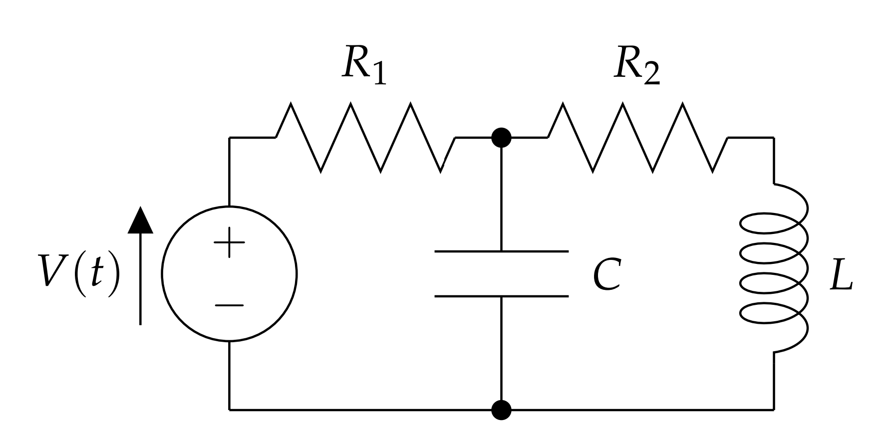
IN THE LAST CHAPTER WE INVESTIGATED SIMPLE SERIES LRC CIRCUITS. More complicated circuits are possible by looking at parallel connections, or other combinations, of resistors, capacitors and inductors. This results in several equations for each loop in the circuit, leading to larger systems of differential equations. An example of another circuit setup is shown in Figure \(\PageIndex{1}\). This is not a problem that can be covered in the first year physics course.

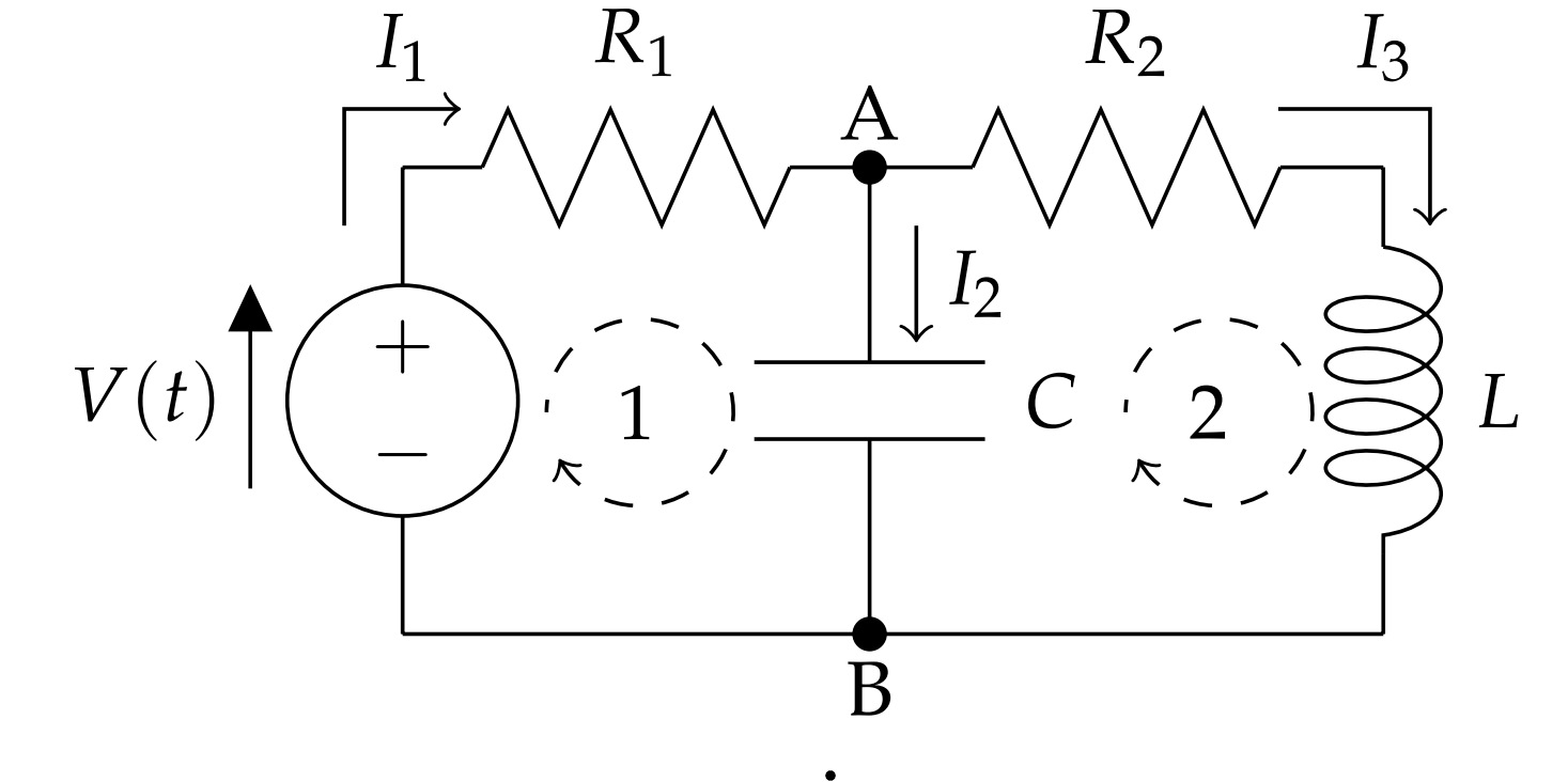
There are two loops, indicated in Figure \(\PageIndex{2}\) as traversed clockwise. For each loop we need to apply Kirchoff’s Loop Rule. There are three oriented currents, labeled \(I_{i}, i=1,2,3\). Corresponding to each current is a changing charge, \(q_{i}\) such that

\[I_{i}=\dfrac{d q_{i}}{d t}, \quad i=1,2,3 \nonumber \]

We have for loop one

\[I_1 R_1 + \dfrac{q_2}{C} = V(t) \nonumber \]

and for loop two

\[I_{3} R_{2}+L \dfrac{d I_{3}}{d t}=\dfrac{q_{2}}{C} . \nonumber \]

Figure \(\PageIndex{1}\): A circuit with two loops containing several different circuit elements.

Figure \(\PageIndex{2}\): The previous parallel circuit with the directions indicated for traversing the loops in Kirchoff’s Laws.

There are three unknown functions for the charge. Once we know the charge functions, differentiation will yield the three currents. However, we only have two equations. We need a third equation. This equation is found from Kirchoff’s Point (Junction) Rule.

Consider the points A and B in Figure \(\PageIndex{2}\). Any charge (current) entering these junctions must be the same as the total charge (current) leaving the junctions. For point \(A\) we have

\[I_{1}=I_{2}+I_{3} \nonumber \]

\[\dot{q}_{1}=\dot{q}_{2}+\dot{q}_{3} \nonumber \]

Equations \(\PageIndex{1}, \PageIndex{2}\), and \(\PageIndex{4}\) form a coupled system of differential equations for this problem. There are both first and second order derivatives involved. We can write the whole system in terms of charges as

\[ \begin{array}{r} R_{1} \dot{q}_{1}+\dfrac{q_{2}}{C}=V(t) \\ R_{2} \dot{q}_{3}+L \ddot{q}_{3}=\dfrac{q_{2}}{C} \\ \dot{q}_{1}=\dot{q}_{2}+\dot{q}_{3} . \end{array} \label{6.49} \]

The question is whether, or not, we can write this as a system of first order differential equations. Since there is only one second order derivative, we can introduce the new variable \(q_{4}=\dot{q}_{3}\). The first equation can be solved for \(\dot{q}_{1}\). The third equation can be solved for \(\dot{q}_{2}\) with appropriate substitutions for the other terms. \(\dot{q}_{3}\) is gotten from the definition of \(q_{4}\) and the second equation can be solved for \(\ddot{q}_{3}\) and substitutions made to obtain the system

\[\begin{aligned} \dot{q}_{1} &=\dfrac{V}{R_{1}}-\dfrac{q_{2}}{R_{1} C} \\ \dot{q}_{2} &=\dfrac{V}{R_{1}}-\dfrac{q_{2}}{R_{1} C}-q_{4} \\ \dot{q}_{3} &=q_{4} \\ \dot{q}_{4} &=\dfrac{q_{2}}{L C}-\dfrac{R_{2}}{L} q_{4} . \end{aligned} \nonumber \]

So, we have a nonhomogeneous first order system of differential equations.