6.2.3: Mixture Problems

There are many types of mixture problems. Such problems are standard in a first course on differential equations as examples of first order differential equations. Typically these examples consist of a tank of brine, water containing a specific amount of salt with pure water entering and the mixture leaving, or the flow of a pollutant into, or out of, a lake. We first saw such problems in Chapter \(1 .\)

In general one has a rate of flow of some concentration of mixture entering a region and a mixture leaving the region. The goal is to determine how much stuff is in the region at a given time. This is governed by the equation

\[\text{Rate of change of substance} = \text{Rate In} - \text{Rate Out}. \nonumber \]

This can be generalized to the case of two interconnected tanks. We will provide an example, but first we review the single tank problem from Chapter \(1 .\)

Example \(\PageIndex{1}\): Single Tank Problem

A 50 gallon tank of pure water has a brine mixture with concentration of 2 pounds per gallon entering at the rate of 5 gallons per minute. [See Figure \(\PageIndex{1}\).] At the same time the well-mixed contents drain out at the rate of 5 gallons per minute. Find the amount of salt in the tank at time \(t .\) In all such problems one assumes that the solution is well mixed at each instant of time.

Figure \(\PageIndex{1}\): A typical mixing problem.

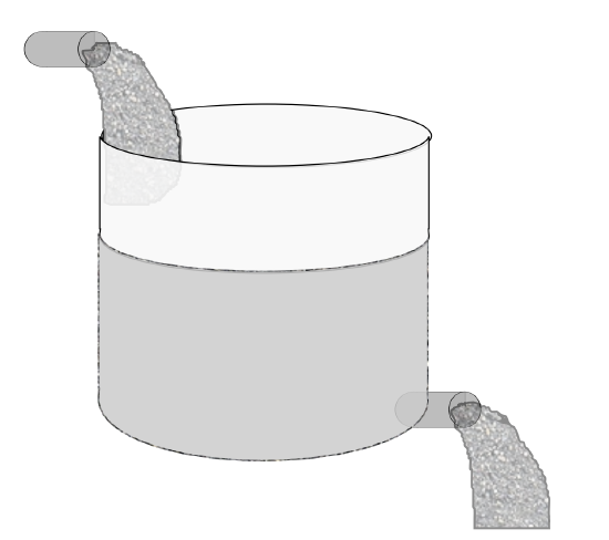
Let \(x(t)\) be the amount of salt at time \(t\). Then the rate at which the salt in the tank increases is due to the amount of salt entering the tank less that leaving the tank. To figure out these rates, one notes that \(d x / d t\) has units of pounds per minute. The amount of salt entering per minute is given by the product of the entering concentration times the rate at which the brine enters. This gives the correct units:

\[\left(2 \dfrac{\text { pounds }}{\text { gal }}\right)\left(5 \dfrac{\text { gal }}{\text { min }}\right)=10 \dfrac{\text { pounds }}{\text { min }}. \nonumber \]

Similarly, one can determine the rate out as

\[\left(\dfrac{x \text { pounds }}{50 \text { gal }}\right)\left(5 \dfrac{\text { gal }}{\text { min }}\right)=\dfrac{x}{10} \dfrac{\text { pounds }}{\text { min }} \nonumber \]

Thus, we have

\[\dfrac{d x}{d t}=10-\dfrac{x}{10} \nonumber \]

This equation is easily solved using the methods for first order equations.

Example \(\PageIndex{2}\): Double Tank Problem

One has two tanks connected together, labeled \(\operatorname{tank} X\) and \(\operatorname{tank} Y\), as shown in Figure \(\PageIndex{2}\).

Figure \(\PageIndex{2}\): The two tank problem.

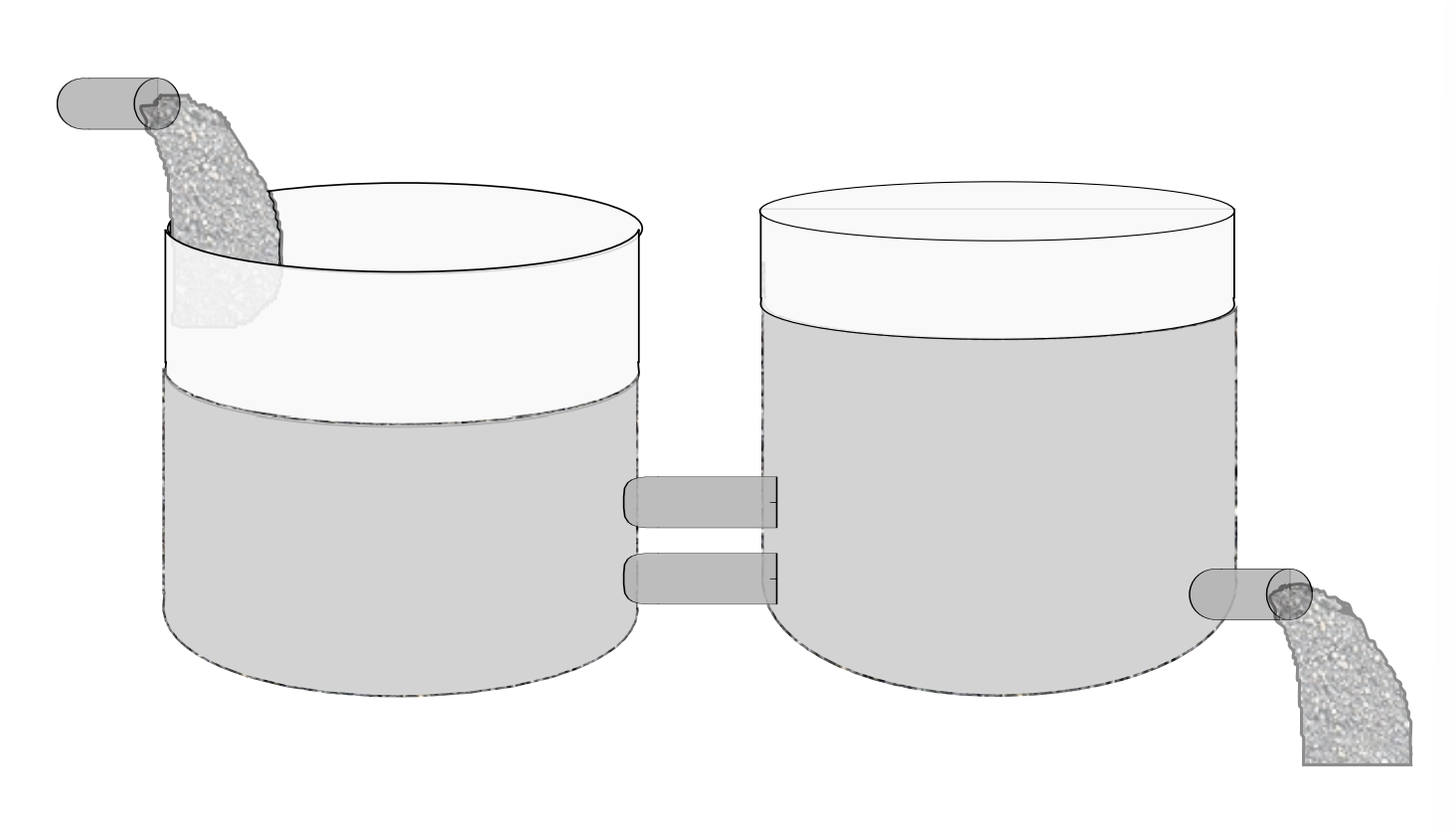
Let tank X initially have 100 gallons of brine made with 100 pounds of salt. Tank Y initially has 100 gallons of pure water. Pure water is pumped into tank \(X\) at a rate of \(2.0\) gallons per minute. Some of the mixture of brine and pure water flows into tank \(Y\) at 3 gallons per minute. To keep the tank levels the same, one gallon of the \(Y\) mixture flows back into \(\tan \mathrm{k} X\) at a rate of one gallon per minute and 2.0 gallons per minute drains out. Find the amount of salt at any given time in the tanks. What happens over a long period of time?

In this problem we set up two equations. Let \(x(t)\) be the amount of salt in \(\operatorname{tank} X\) and \(y(t)\) the amount of salt in tank \(Y\). Again, we carefully look at the rates into and out of each tank in order to set up the system of differential equations. We obtain the system

\[ \begin{aligned} \dfrac{d x}{d t} &=\dfrac{y}{100}-\dfrac{3 x}{100} \\ \dfrac{d y}{d t} &=\dfrac{3 x}{100}-\dfrac{3 y}{100} \end{aligned} \label{6.50} \]

This is a linear, homogenous constant coefficient system of two first order equations, which we know how to solve. The matrix form of the system is given by

\[\dot{\mathbf{x}}=\left(\begin{array}{cc} -\dfrac{3}{100} & \dfrac{1}{100} \\ \dfrac{3}{100} & -\dfrac{3}{100} \end{array}\right) \mathbf{x}, \quad \mathbf{x}(0)=\left(\begin{array}{c} 100 \\ 0 \end{array}\right)\nonumber \]

The eigenvalues for the problem are given by \(\lambda=-3 \pm \sqrt{3}\) and the eigenvectors are

\[\left(\begin{array}{c} 1 \\ \pm \sqrt{3} \end{array}\right) \nonumber \]

Since the eigenvalues are real and distinct, the general solution is easily written down:

\[\mathbf{x}(t)=c_{1}\left(\begin{array}{c} 1 \\ \sqrt{3} \end{array}\right) e^{(-3+\sqrt{3}) t}+c_{2}\left(\begin{array}{c} 1 \\ -\sqrt{3} \end{array}\right) e^{(-3-\sqrt{3}) t} \nonumber \]

Finally, we need to satisfy the initial conditions. So,

\[\mathbf{x}(0)=c_{1}\left(\begin{array}{c} 1 \\ \sqrt{3} \end{array}\right)+c_{2}\left(\begin{array}{c} 1 \\ -\sqrt{3} \end{array}\right)=\left(\begin{array}{c} 100 \\ 0 \end{array}\right),\nonumber \]

or

\[c_{1}+c_{2}=100, \quad\left(c_{1}-c_{2}\right) \sqrt{3}=0.\nonumber \]

So, \(c_{2}=c_{1}=50\). The final solution is

\[\mathbf{x}(t)=50\left(\left(\begin{array}{c} 1 \\ \sqrt{3} \end{array}\right) e^{(-3+\sqrt{3}) t}+\left(\begin{array}{c} 1 \\ -\sqrt{3} \end{array}\right) e^{(-3-\sqrt{3}) t}\right),\nonumber \]

or

\[ \begin{aligned} &x(t)=50\left(e^{(-3+\sqrt{3}) t}+e^{(-3-\sqrt{3}) t}\right) \\ &y(t)=50 \sqrt{3}\left(e^{(-3+\sqrt{3}) t}-e^{(-3-\sqrt{3}) t}\right) . \end{aligned} \label{6.51} \]