7.6: Nonlinear Population Models

WE HAVE ALREADY ENCOUNTERED SEVERAL MODELS Of population dynamics in this and previous chapters. Of course, one could dream up several other examples. While such models might seem far from applications in physics, it turns out that these models lead to systems od differential equations which also appear in physical systems such as the coupling of waves in lasers, in plasma physics, and in chemical reactions.

The Lotka-Volterra model is named after model looks similar, except there are a few sign changes, since one species Alfred James Lotka (188o-1949) and Vito Volterra (1860-1940). is not feeding on the other. Also, we can build in logistic terms into our model. We will save this latter type of model for the homework.

Two well-known nonlinear population models are the predator-prey and competing species models. In the predator-prey model, one typically has one species, the predator, feeding on the other, the prey. We will look at the standard Lotka-Volterra model in this section. The competing species

(The Lotka-Volterra model of population dynamics). The Lotka-Volterra model takes the form

\[ \begin{aligned} & \dot{x}=a x-b x y, \\ & \dot{y}=-d y+c x y, \end{aligned} \label{7.36} \]

where \(a, b, c\), and \(d\) are positive constants. In this model, we can think of \(x\) as the population of rabbits (prey) and \(y\) is the population of foxes (predators). Choosing all constants to be positive, we can describe the terms.

• \(ax\): When left alone, the rabbit population will grow. Thus \(a\) is the natural growth rate without predators.
• \(-d y\): When there are no rabbits, the fox population should decay. Thus, the coefficient needs to be negative.
• \(-bxy\): We add a nonlinear term corresponding to the depletion of the rabbits when the foxes are around.
• \(cxy\): The more rabbits there are, the more food for the foxes. So, we add a nonlinear term giving rise to an increase in fox population.

Example \(\PageIndex{1}\)

Determine the equilibrium points and their stability for the Lotka-Volterra system.

The analysis of the Lotka-Volterra model begins with determining the fixed points. So, we have from Equation \(\PageIndex{1}\)

\[ \begin{aligned} x(a-b y) &=0, \\ y(-d+c x) &=0 . \end{aligned} \label{7.37} \]

Therefore, the origin, \((0,0)\), and \(\left(\dfrac{d}{c}, \dfrac{a}{b}\right)\) are the fixed points.

Next, we determine their stability, by linearization about the fixed points. We can use the Jacobian matrix, or we could just expand the right-hand side of each equation in Equation \(\PageIndex{1}\) about the equilibrium points as shown in he next example. The Jacobian matrix for this system is

\[\operatorname{Df}(x, y)=\left(\begin{array}{cc} a-b y & -b x \\ c y & -d+c x \end{array}\right) \nonumber \]

Evaluating at each fixed point, we have

\[D f(0,0)=\left(\begin{array}{cc} a & 0 \\ 0 & -d \end{array}\right) , \nonumber \]

\[D f\left(\dfrac{d}{c}, \dfrac{a}{b}\right)=\left(\begin{array}{cc} 0 & -\dfrac{b d}{c} \\ \dfrac{a c}{b} & 0 \end{array}\right) . \nonumber \]

The eigenvalues of \(\left(7 \cdot 3^{8}\right)\) are \(\lambda=a,-d .\) So, the origin is a saddle point.

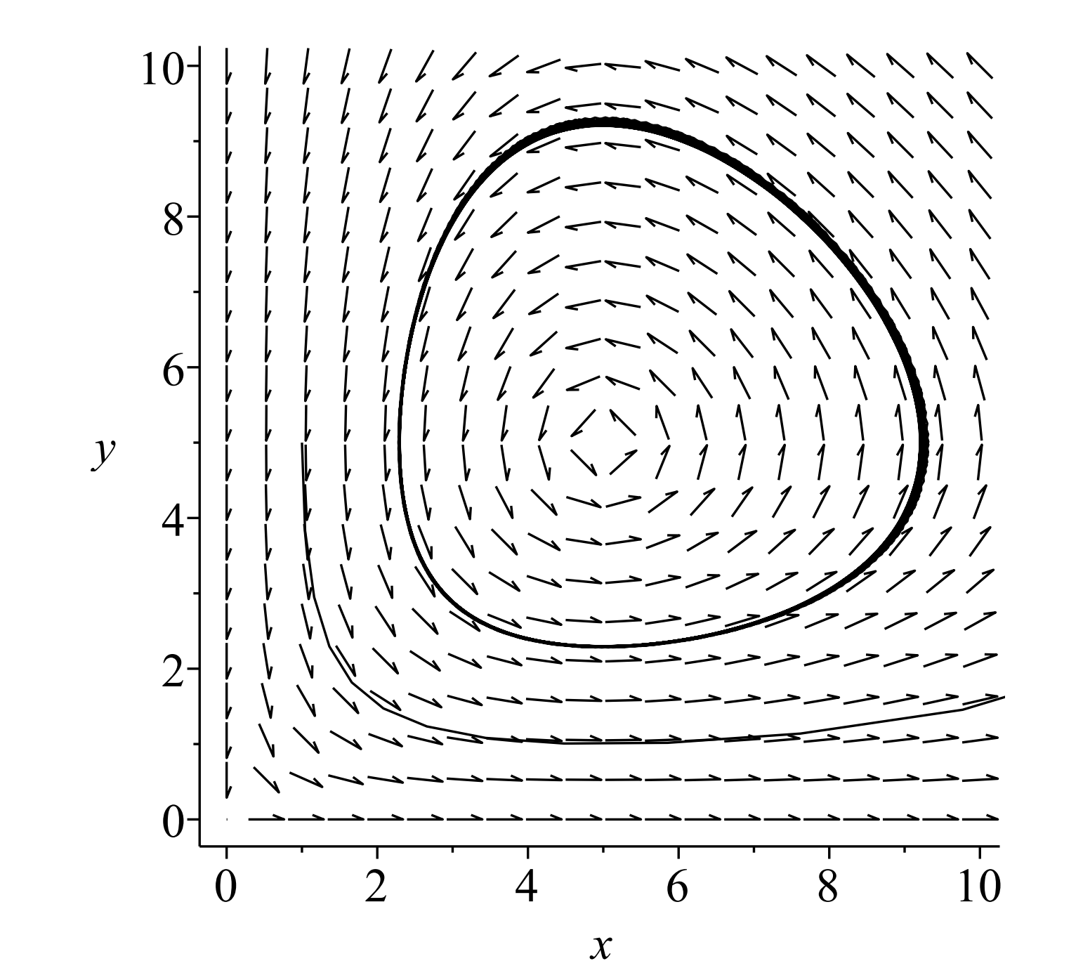
The eigenvalues of Equation \(\PageIndex{4}\) satisfy \(\lambda^{2}+a d=0 .\) So, the other point is a center. In Figure \(\PageIndex{1}\) we show a sample direction field for the Lotka-Volterra system.

Figure \(\PageIndex{1}\):Phase plane for the LotkaVolterra system given by \(\dot{x}=x-0.2 x y\), \(\dot{y}=-y+0.2 x y\). Solution curves are shown for initial conditions \(\left(x_{0}, y_{0}\right)=\) \((8,3),(1,5)\).

Another way to carry out the linearization of the system of differential equations is to expand the equations about the fixed points. For fixed points \((x^{*}, y^{*})\), we let

\[(x, y)=\left(x^{*}+u, y^{*}+v\right) \nonumber \]

Inserting this translation of the origin into the equations of the system, and dropping nonlinear terms in \(u\) and \(v\), results in the linearized system. This method is equivalent to analyzing the Jacobian matrix for each fixed point.

Direct linearization of a system is carried out by introducing \(\mathbf{x}=\mathbf{x}^{*}+\xi\), or \((x, y)=\left(x^{*}+u, y^{*}+v\right)\) into the system and dropping nonlinear terms in \(u\) and \(v\).

Example \(\PageIndex{1}\)

Expand the Lotka-Volterra system about the equilibrium points.

For the origin \((0,0)\) the linearization about the origin amounts to simply dropping the nonlinear terms. In this case we have

\[ \begin{aligned}
&\dot{u}=a u, \\
&\dot{v}=-d v .
\end{aligned}\label{7.40} \]

The coefficient matrix for this system is the same as \(D f(0, 0)\).

For the second fixed point, we let

\[(x,y)=\dfrac{d}{c}+u, \dfrac{a}{b} +v\). \nonumber \]

Inserting this transformation into the system gives

\[ \begin{aligned}
\dot{u} &=a\left(\frac{d}{c}+u\right)-b\left(\frac{d}{c}+u\right)\left(\frac{a}{b}+v\right) \\
\dot{v} &=-d\left(\frac{a}{b}+v\right)+c\left(\frac{d}{c}+u\right)\left(\frac{a}{b}+v\right) .
\end{aligned} \label{7.41} \]

Expanding, we obtain

\[ \begin{aligned} \dot{u} &=\dfrac{a d}{c}+a u-b\left(\dfrac{a d}{b c}+\dfrac{d}{c} v+\dfrac{a}{b} u+u v\right) \\ \dot{v} &=-\dfrac{a d}{b}-d v+c\left(\dfrac{a d}{b c}+\dfrac{d}{c} v+\dfrac{a}{b} u+u v\right) \end{aligned} \label{7.42} \]

In both equations the constant terms cancel and linearization is simply getting rid of the \(u v\) terms. This leaves the linearized system

\[ \begin{aligned} \dot{u} &=a u-b\left(\dfrac{d}{c} v+\dfrac{a}{b} u\right) \\ \dot{v} &=-d v+c\left(+\dfrac{d}{c} v+\dfrac{a}{b} u\right) \end{aligned}\label{7.43} \]

Or

\[ \begin{aligned} \dot{u} &=-\dfrac{b d}{c} v, \\ \dot{v} &=\dfrac{a c}{b} u . \end{aligned} \label{7.44} \]

The coefficient matrix for this linearized system is the same as \(D f\left(\dfrac{d}{c}, \dfrac{a}{b}\right)\). In fact, for nearby orbits, they are almost circular orbits. From this linearized system, we have \(\ddot{u}+a d u=0\).

We can take \(u=A \cos (\sqrt{a d} t+\phi)\), where \(A\) and \(\phi\) can be determined from the initial conditions. Then,

\[ \begin{aligned} v &=-\dfrac{c}{b d} \dot{u} \\ &=\dfrac{c}{b d} A \sqrt{a d} \sin (\sqrt{a d} t+\phi) \\ &=\dfrac{c}{b} \sqrt{\dfrac{a}{d}} A \sin (\sqrt{a d} t+\phi) \end{aligned} \label{7.45} \]

Therefore, the solutions near the center are given by

\[(x, y)=\left(\dfrac{d}{c}+A \cos (\sqrt{a d} t+\phi), \dfrac{a}{b}+\dfrac{c}{b} \sqrt{\dfrac{a}{d}} A \sin (\sqrt{a d} t+\phi)\right). \nonumber \]

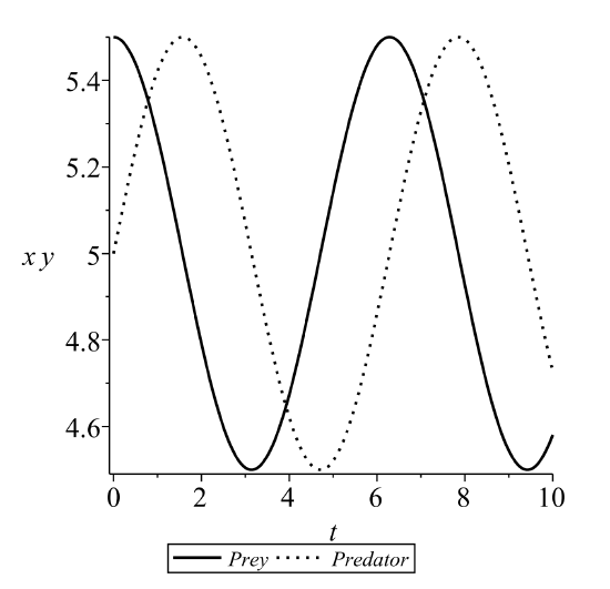
For \(a=d=1, b=c=0.2\), and initial values of \(\left(x_{0}, y_{0}\right)=(5.5,5)\), these solutions become

\[x(t)=5.0+0.5 \cos t, \quad y(t)=5.0+0.5 \sin t\nonumber \]

Plots of these solutions are shown in Figure \(\PageIndex{2}\).

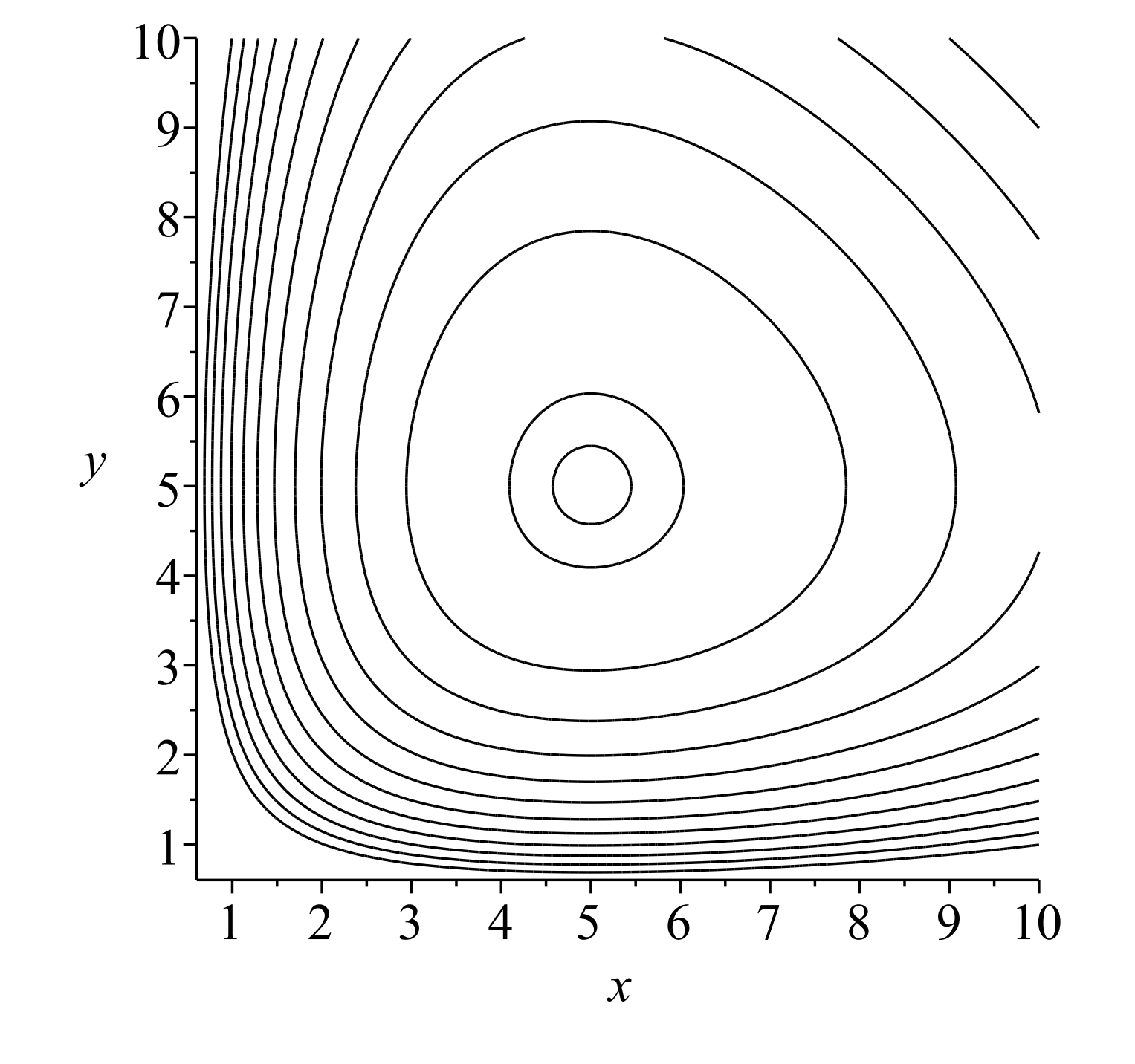
It is also possible to find a first integral of the Lotka-Volterra system whose level curves give the phase portrait of the system. As we had done in Chapter 2, we can write

\[\begin{aligned} \dfrac{d y}{d x} &=\dfrac{\dot{y}}{\dot{x}} \\ &=\dfrac{-d y+c x y}{a x-b x y} \\ &=\dfrac{y(-d+c x)}{x(a-b y)} \end{aligned} \label{7.46} \]

Figure \(\PageIndex{2}\): The linearized solutions of Lotka-Volterra system \(\dot{x}=x-0.2 x y\), \(\dot{y}=-y+0.2 x y\) for the initial conditions \(\left(x_{0}, y_{0}\right)=(5.5,5)\).

This is an equation of the form seen in Problem 2.6.13. This equation is now a separable differential equation. The solution this differential equation is given in implicit form as

\[a ln y + d ln x − cx − by = C \nonumber \]

,

where \(C\) is an arbitrary constant. This expression is known as the first system.

Figure \(\PageIndex{3}\): Phase plane for the LotkaVolterra system given by \(\dot{x}=x-0.2 x y\), \(\dot{y}=-y+0.2 x y\) based upon the first integral of the system.