
7.7: Limit Cycles


- Last updated
- May 24, 2024
- Save as PDF

( \newcommand{\kernel}{\mathrm{null}\,}\)
So far we have just been concerned with equilibrium solutions and their behavior. However, asymptotically stable fixed points are not the only attractors. There are other types of solutions, known as limit cycles, towards which a solution may tend. In this section we will look at some examples of these periodic solutions.
Such solutions are common in nature. Rayleigh investigated the problem
x′′+c(13(x′)2−1)x′+x=0
in the study of the vibrations of a violin string. Balthasar van der Pol (1889-1959) studied an electrical circuit, modeling this behavior. Others have looked into biological systems, such as neural systems, chemical reactions, such as Michaelis-Menten kinetics, and other chemical systems leading to chemical oscillations. One of the most important models in the historical study of dynamical systems is that of planetary motion and investigating the stability of planetary orbits. As is well known, these orbits are periodic.
Limit cycles are isolated periodic solutions towards which neighboring states might tend when stable. A key example exhibiting a limit cycle is given in the next example.
Find the limit cycle in the system
x′=μx−y−x(x2+y2)y′=x+μy−y(x2+y2)
Solution
It is clear that the origin is a fixed point. The Jacobian matrix is given as
Df(0,0)=(μ−11μ)
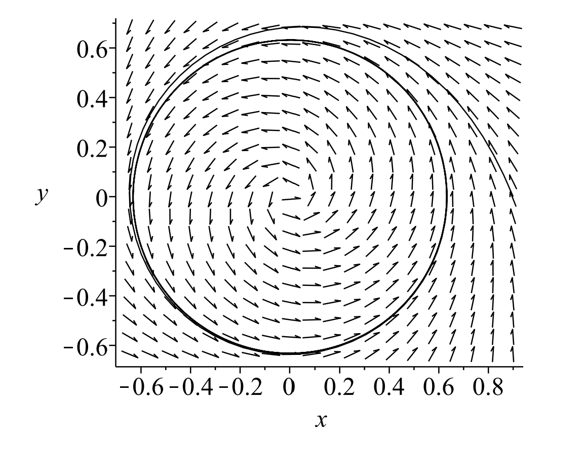
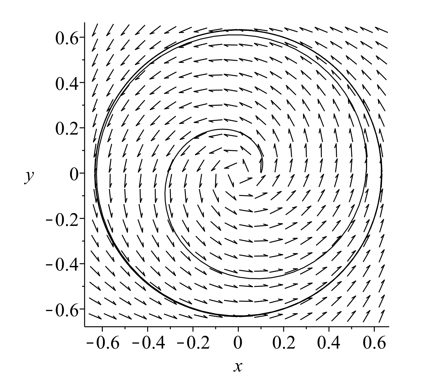
The eigenvalues are found to be λ=μ±i. For μ=0 we have a center. For μ<0 we have a stable spiral and for μ>0 we have an unstable spiral. However, this spiral does not wander off to infinity. We see in Figure 7.7.1 that the equilibrium point is a spiral. However, in Figure 7.7.2 it is clear that the solution does not spiral out to infinity. It is bounded by a circle.
One can actually find the radius of this circle. This requires rewriting the system in polar form. Recall from Chapter 2 that we can change derivatives of Cartesian coordinates to derivatives of polar coordinates by using the relations
rr′=xx′+yy′
r2θ′=xy′−yx′
Inserting the system 7.7.2 into these expressions, we have
rr′=μr2−r4,r2θ′=r2.
This leads to the system
r′=μr−r3,θ′=1.
Of course, for a circle the radius is constant, r= const. Therefore, in order to find the limit cycle, we need to look at the equilibrium solutions of Equation 7.7.6. This amounts to finding the constant solutions of μr−r3=0. The equilibrium solutions are r=0,±√μ. The limit cycle corresponds to the positive radius solution, r=√μ.
In Figures 7.7.1−7.7.2 we take μ=0.4. In this case we expect a circle with r=√0.4≈0.63. From the θ equation, we have that θ′>0. This means that we follow the limit cycle in a counterclockwise direction as time increases.
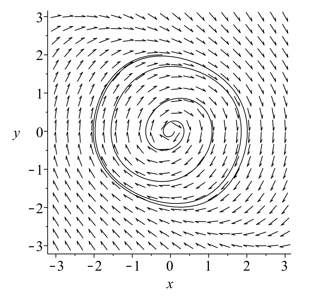
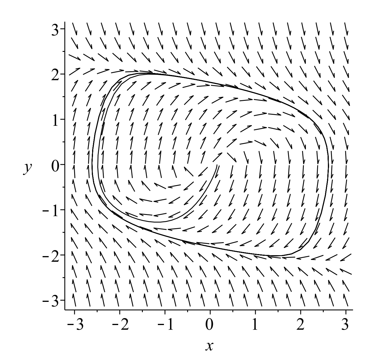
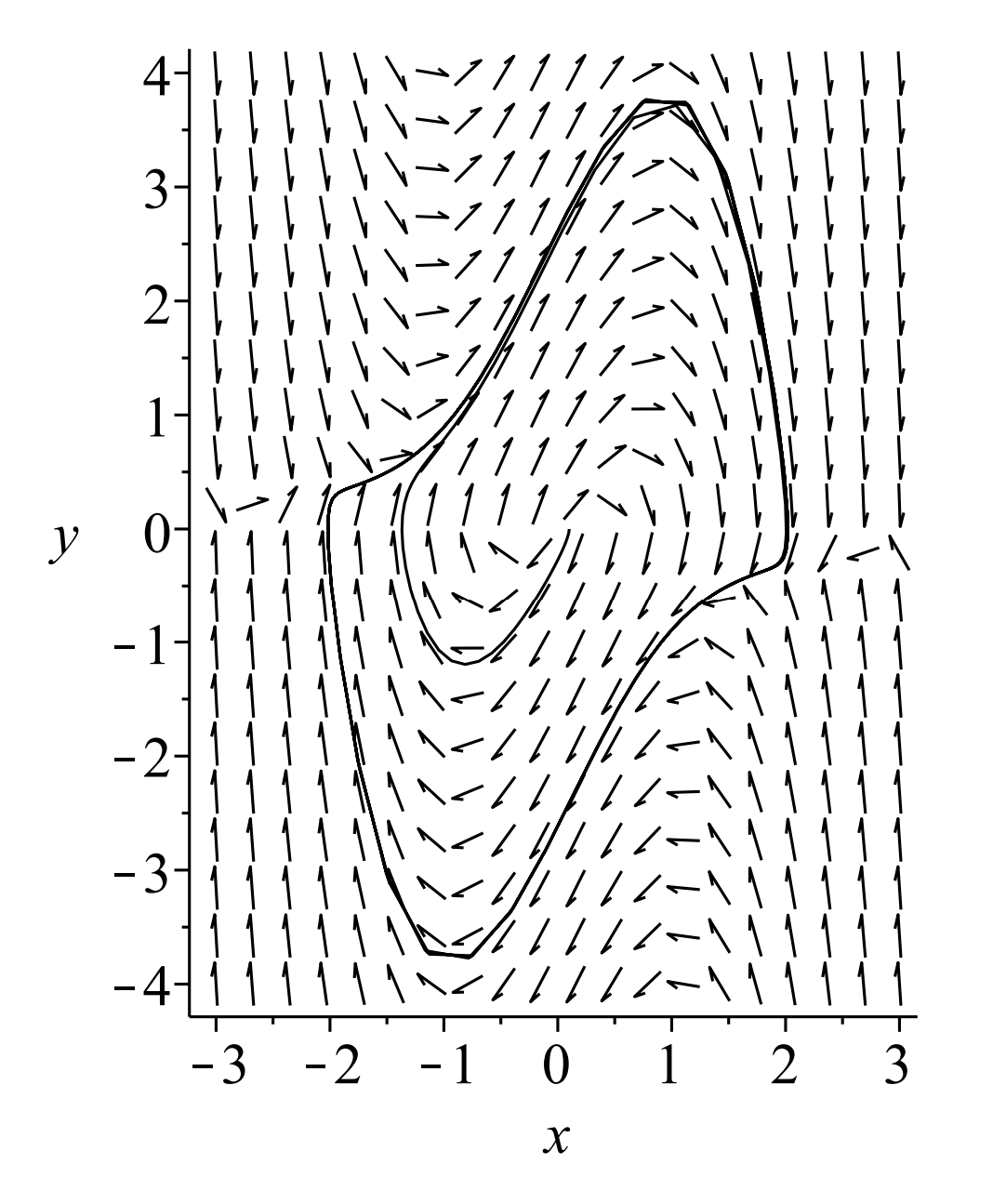
Limit cycles are not always circles. In Figures 7.7.3−7.7.4 we show the behavior of the Rayleigh system 7.7.1 for c=0.4 and c=2.0. In this case we see that solutions tend towards a noncircular limit cycle in a clockwise direction.
A slight change of the Rayleigh system leads to the van der Pol equation:
x′′+c(x2−1)x′+x=0
(The van der Pol system). The limit cycle for c=2.0 is shown in Figure 7.7.5.
Can one determine ahead of time if a given nonlinear system will have a limit cycle? In order to answer this question, we will introduce some definitions.
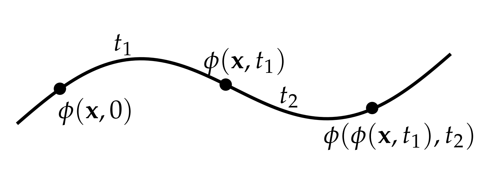
We first describe different trajectories and families of trajectories. A flow on R2 is a function ϕ that satisfies the following
- ϕ(x,t) is continuous in both arguments.
- ϕ(x,0)=x for all x∈R2.
- ϕ(ϕ(x,t1),t2)=ϕ(x,t1+t2).
(Orbits and trajectories). The orbit, or trajectory, through x is defined as γ={ϕ(x,t)∣t∈I}. In Figure 7.7.6 we demonstrate these properties. For t=0,ϕ(x,0)=x. Increasing t, one follows the trajectory until one reaches the point ϕ(x,t1). Continuing t2 further, one is then at ϕ(ϕ(x,t1),t2). By the third property, this is the same as going from x to ϕ(x,t1+t2) for t=t1+t2.
Having defined the orbits, we need to define the asymptotic behavior of the orbit for both positive and negative large times. We define the positive semiorbit through x as γ+={ϕ(x,t)∣t>0}. The negative semiorbit through x is defined as γ−={ϕ(x,t)∣t<0}. Thus, we have γ=γ+∪γ−.
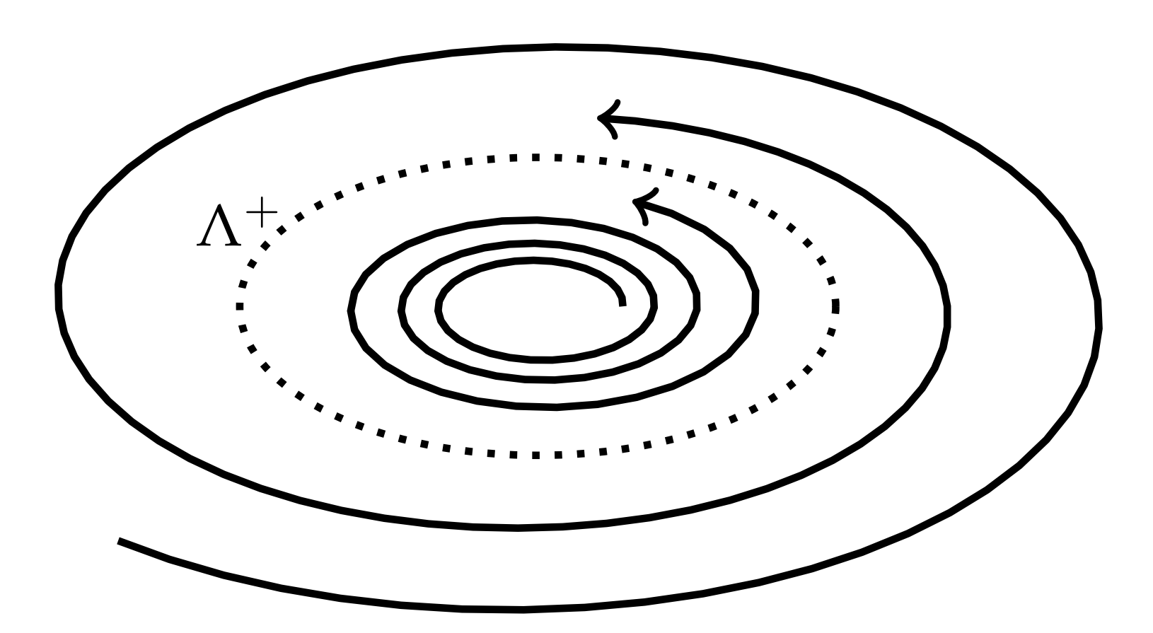
(Limit sets and limit points). The positive limit set, or w-limit set, of point x is defined as
Λ+={y∣ there exists a sequence of tn→∞ such that ϕ(x,tn)→y}
The y′ s are referred to as w-limit points. This is shown in Figure 7.7.7.
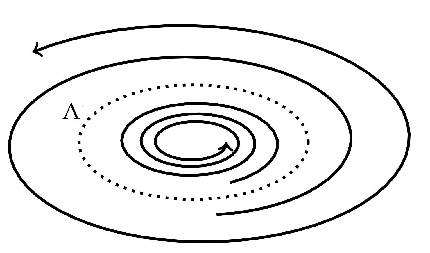
Similarly, we define the negative limit set, or the alpha-limit set, of point x is defined as
Λ−={y∣ there exists a sequences of tn→−∞ such that ϕ(x,tn)→y}
and the corresponding y′ s are α-limit points. This is shown in Figure 7.7.8.
(Cycles and periodic orbits). There are several types of orbits that a system might possess. A cycle or periodic orbit is any closed orbit which is not an equilibrium point. A periodic orbit is stable if for every neighborhood of the orbit such that all nearby orbits stay inside the neighborhood. Otherwise, it is unstable. The orbit is asymptotically stable if all nearby orbits converge to the periodic orbit.
A limit cycle is a cycle which is the α or ω-limit set of some trajectory other than the limit cycle. A limit cycle Γ is stable if Λ+=Γ for all x in some neighborhood of Γ. A limit cycle Γ is unstable if Λ−=Γ for all x in some neighborhood of Γ. Finally, a limit cycle is semistable if it is attracting on one side and repelling on the other side. In the previous examples, we saw limit cycles that were stable. Figures 7.7.7 and 7.7.8depict stable and unstable limit cycles, respectively.
We now state a theorem which describes the type of orbits we might find in our system.
Let γ+be contained in a bounded region in which there are finitely many critical points. Then Λ+is either
- a single critical point;
- a single closed orbit;
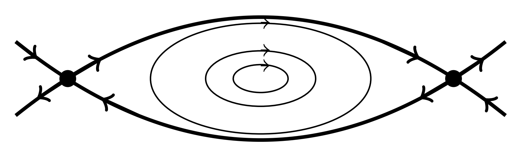
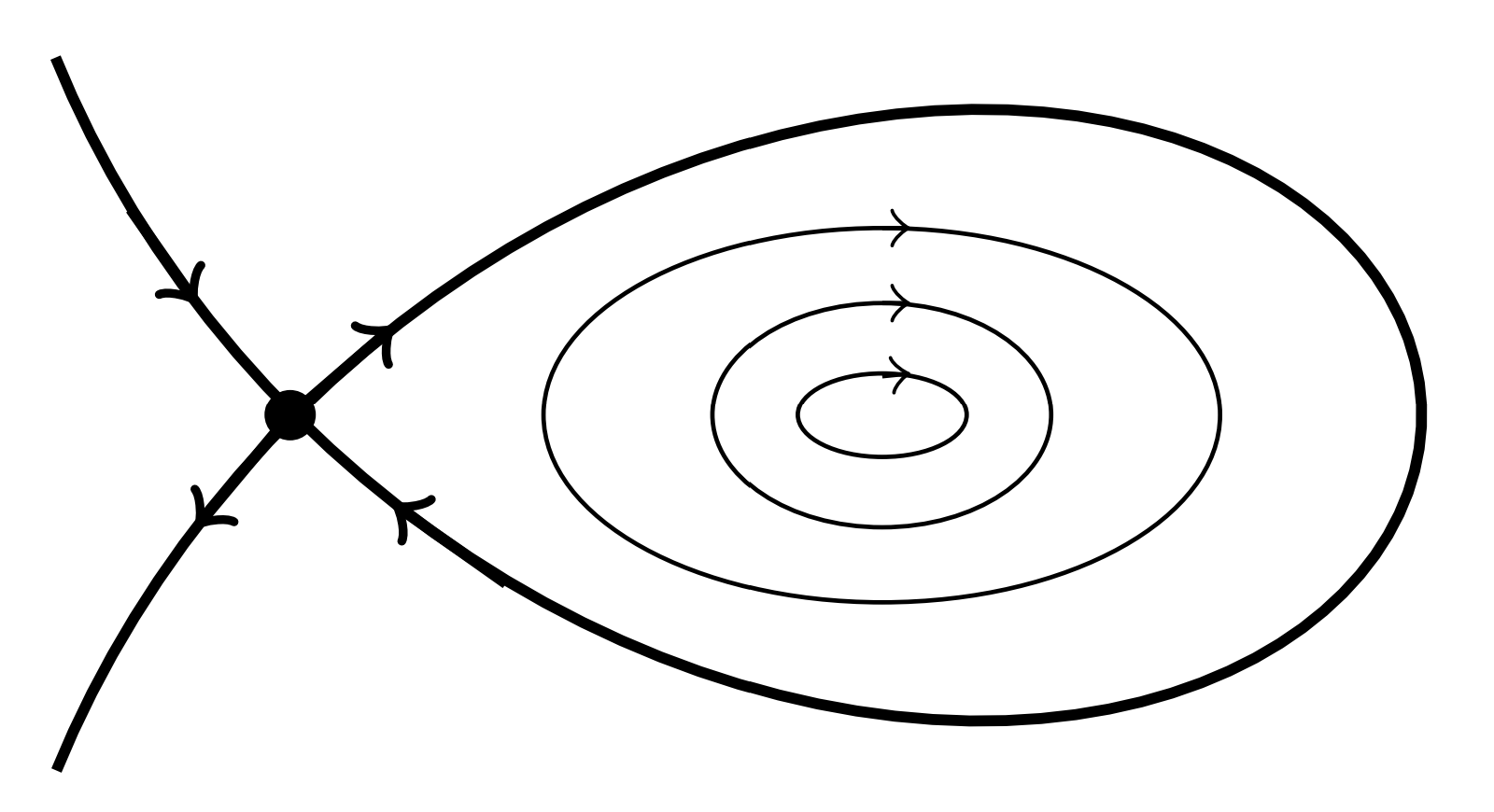
- a set of critical points joined by heteroclinic orbits. [Compare Figures 7.7.9 and 7.7.10. ]
We are interested in determining when limit cycles may, or may not, exist. A consequence of the Poincaré-Bendixon Theorem is given by the following corollary.
Let D be a bounded closed set containing no critical points and suppose that γ+⊂D. Then there exists a limit cycle contained in D.
More specific criteria allow us to determine if there is a limit cycle in a given region. These are given by Dulac’s Criteria and Bendixon’s Criteria.
Consider the autonomous planar system
x′=f(x,y),y′=g(x,y)
and a continuously differentiable function ψ def
D contained in some open set. If
∂∂x(ψf)+∂∂y(ψg)
does not change sign in D, then there is at most one limit cycle contained entirely in D.
Consider the autonomous planar system
x′=f(x,y),y′=g(x,y)
defined on a simply connected domain D such that
∂∂x(ψf)+∂∂y(ψg)≠0
in D. Then, there are no limit cycles entirely in D.
- Proof.
-
These are easily proved using Green’s Theorem in the Plane. (See your calculus text.) We prove Bendixon’s Criteria. Let f=(f,g). Assume that Γ is a closed orbit lying in D. Let S be the interior of Γ. Then
∫S∇⋅fdxdy=∮Γ(fdy−gdx)=∫T0(f˙y−g˙x)dt=∫T0(fg−gf)dt=0.
So, if ∇⋅f is not identically zero and does not change sign in S, then from the continuity of ∇⋅f in S we have that the right side above is either positive or negative. Thus, we have a contradiction and there is no closed orbit lying in D.
Consider the earlier example in (7⋅48) with μ=1.
x′=x−y−x(x2+y2)y′=x+y−y(x2+y2)
We already know that a limit cycle exists at x2+y2=1. A simple computation gives that
∇⋅f=2−4x2−4y2
For an arbitrary annulus a<x2+y2<b, we have
2−4b<∇⋅f<2−4a
For a=3/4 and b=5/4,−3<∇⋅f<−1. Thus, ∇⋅f<0 in the annulus 3/4<x2+y2<5/4. Therefore, by Dulac’s Criteria there is at most one limit cycle in this annulus.
Consider the system
x′=yy′=−ax−by+cx2+dy2.
Let ψ(x,y)=e−2dx. Then,
∂∂x(ψy)+∂∂y(ψ(−ax−by+cx2+dy2))=−be−2dx≠0
We conclude by Bendixon’s Criteria that there are no limit cycles for this system.