7.8: Nonautonomous Nonlinear Systems

IN THIS SECTION WE DISCUSS NONAUTONOMOUS SYSTEMS. Recall that an autonomous system is one in which there is no explicit time dependence. A simple example is the forced nonlinear pendulum given by the nonhomogeneous equation

\[\ddot{x}+\omega^{2} \sin x=f(t) \nonumber \]

We can set this up as a system of two first order equations:

\[ \begin{aligned} &\dot{x}=y \\ &\dot{y}=-\omega^{2} \sin x+f(t) . \end{aligned} \label{7.58} \]

This system is not in a form for which we could use the earlier methods. Namely, it is a nonautonomous system. However, we introduce a new variable \(z(t)=t\) and turn it into an autonomous system in one more dimension. The new system takes the form

\[ \begin{aligned} \dot{x} &=y \\ \dot{y} &=-\omega^{2} \sin x+f(z) . \\ \dot{z} &=1 . \end{aligned} \label{7.59} \]

The system is now a three dimensional autonomous, possibly nonlinear, system and can be explored using methods from Chapters 2 and 3 .

A more interesting model is provided by the Duffing Equation. This equation, named after Georg Wilhelm Christian Caspar Duffing (1861-1944), models hard spring and soft spring oscillations. It also models a periodically forced beam as shown in Figure \(\PageIndex{1}\). It is of interest because it is a simple equation describes a periodically forced new visualization methods for nonautonomous systems.

Figure \(\PageIndex{1}\): One model of the Duffing equation describes a periodically forced beam which interacts with two magnets.

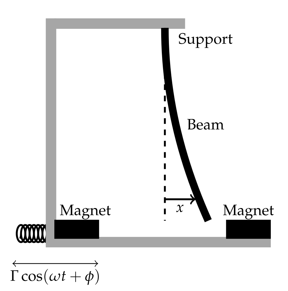
The most general form of Duffing’s equation is given by the damped, forced system

\[\ddot{x}+k \dot{x}+\left(\beta x^{3} \pm \omega_{0}^{2} x\right)=\Gamma \cos (\omega t+\phi) . \nonumber \]

This equation models hard spring, \((\beta>0)\), and soft spring, \((\beta<0)\), oscillations. However, we will use the simpler version of the Duffing equation:

\[\ddot{x}+k \dot{x}+x^{3}-x=\Gamma \cos \omega t . \nonumber \]

An equation of this form can be obtained by setting \(\phi=0\) and rescaling \(x\) and \(t\) in the original equation. We will explore the behavior of the system as we vary the remaining parameters. In Figures \(\PageIndex{2}-\PageIndex{5}\) we show some typical solution plots superimposed on the direction field.

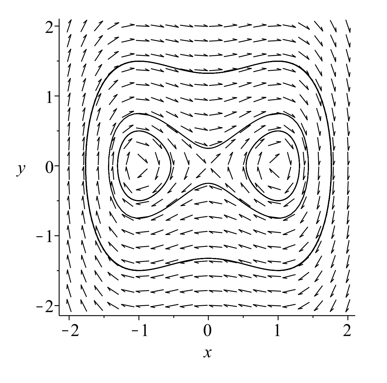
(The undamped, unforced Duffing equation). We start with the undamped \((k=0)\) and unforced \((\Gamma=0)\) Duffing equation,

\[\ddot{x}+x^{3}-x=0 \nonumber \]

We can write this second order equation as the autonomous system

\[ \begin{aligned} \dot{x} &=y \\ \dot{y} &=x\left(1-x^{2}\right) . \end{aligned} \label{7.62} \]

We see that there are three equilibrium points at \((0,0)\) and \((\pm 1,0) .\) In Figure \(\PageIndex{3}\) we plot several orbits for \(k=0\), and \(\Gamma=0\). We see that the three equilibrium points consist of two centers and a saddle.

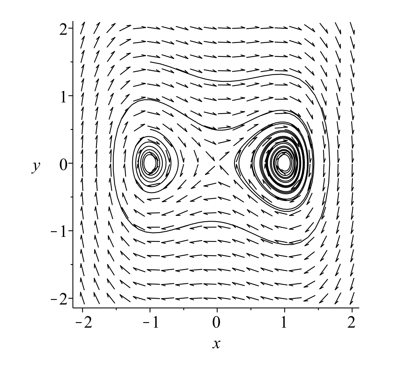
(The unforced Duffing equation). We now turn on the damping. The system becomes

\[ \begin{aligned} \dot{x} &=y \\ \dot{y} &=-k y+x\left(1-x^{2}\right) . \end{aligned} \label{7.63} \]

In Figures \(\PageIndex{3}\) and \(\PageIndex{4}\) we show what happens when \(k=0.1\). These plots are reminiscent of the plots for the nonlinear pendulum; however, there are fewer equilibria. Note that the centers become stable spirals for \(k>0\).

Figure \(\PageIndex{2}\): Phase plane for the undamped, unforced Duffing equation \((k=0, \Gamma=0)\).

Figure \(\PageIndex{3}\): Phase plane for the unforced Duffing equation with \(k=0.1\) and \(\Gamma=0\).

Next we turn on the forcing to obtain a damped, forced Duffing equation. The system is now nonautonomous.

The damped, forced Duffing equation.

\[ \begin{aligned} \dot{x} &=y \\ \dot{y} &=x\left(1-x^{2}\right)+\Gamma \cos \omega t . \end{aligned} \label{7.64} \]

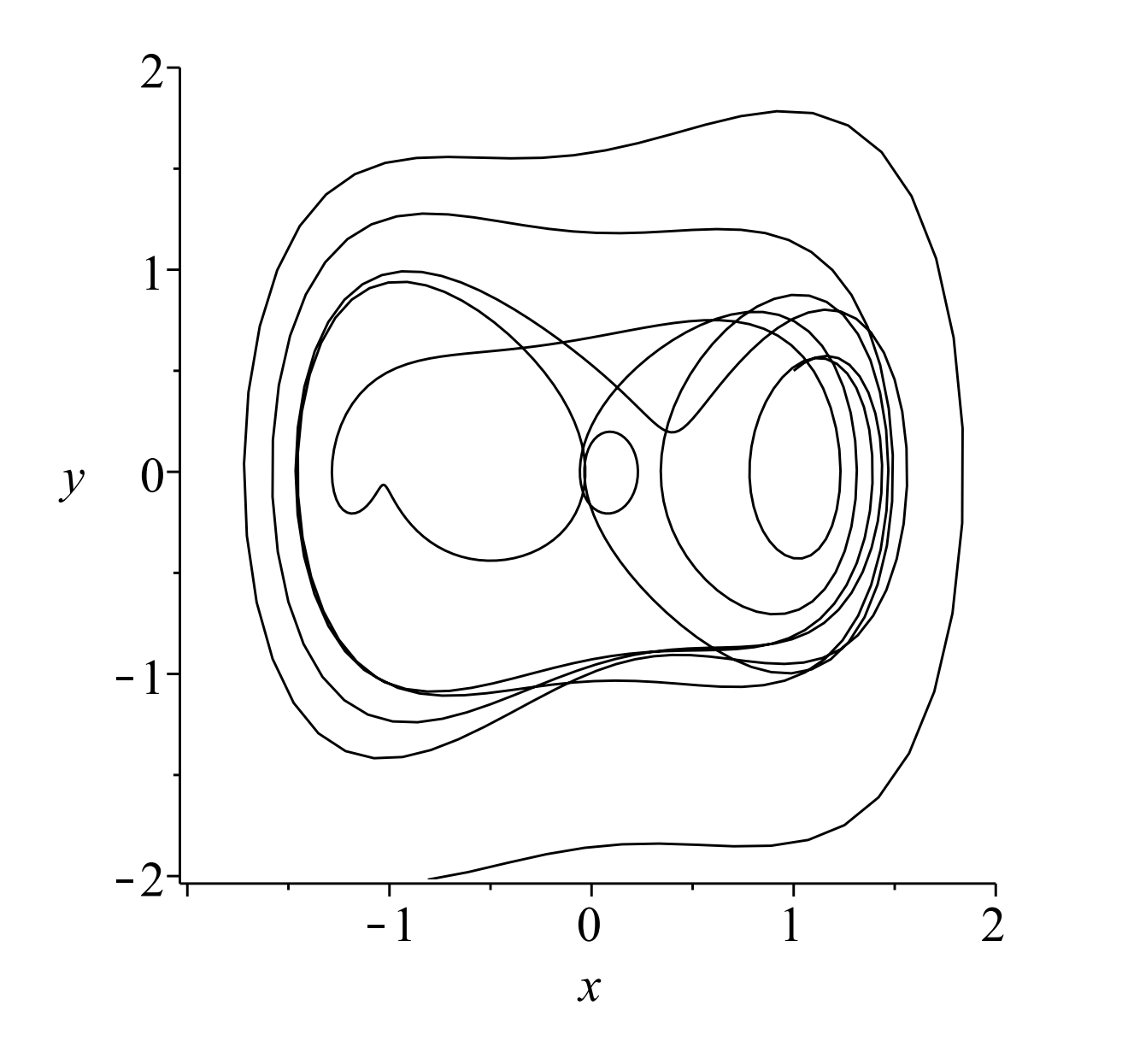
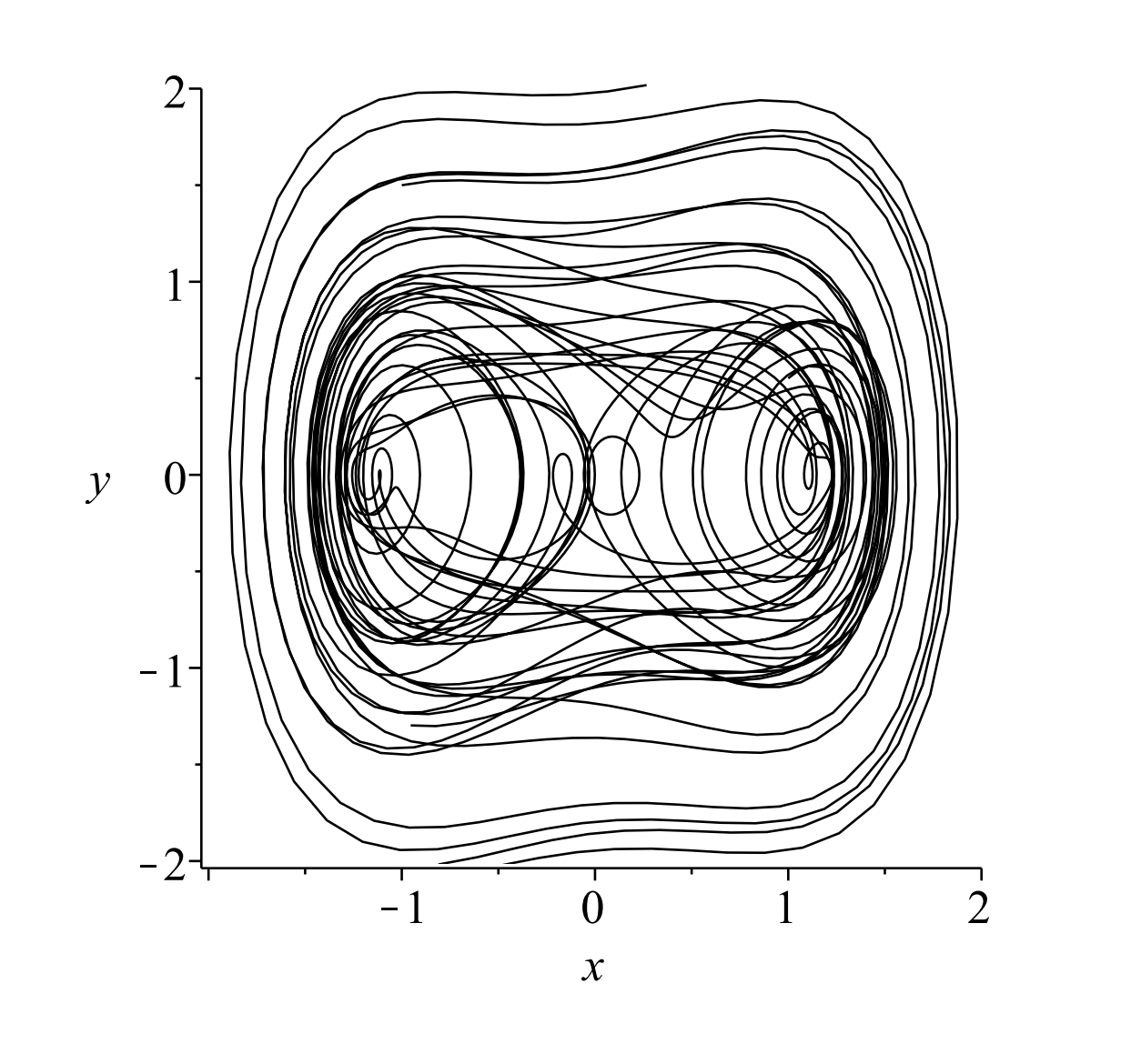
In Figure \(\PageIndex{5}\) we only show one orbit with \(k=0.1, \Gamma=0.5\), and \(\omega=1.25\). The solution intersects itself and look a bit messy. We can imagine what we would get if we added any more orbits. For completeness, we show in Figure \(\PageIndex{6}\) an example with four different orbits.

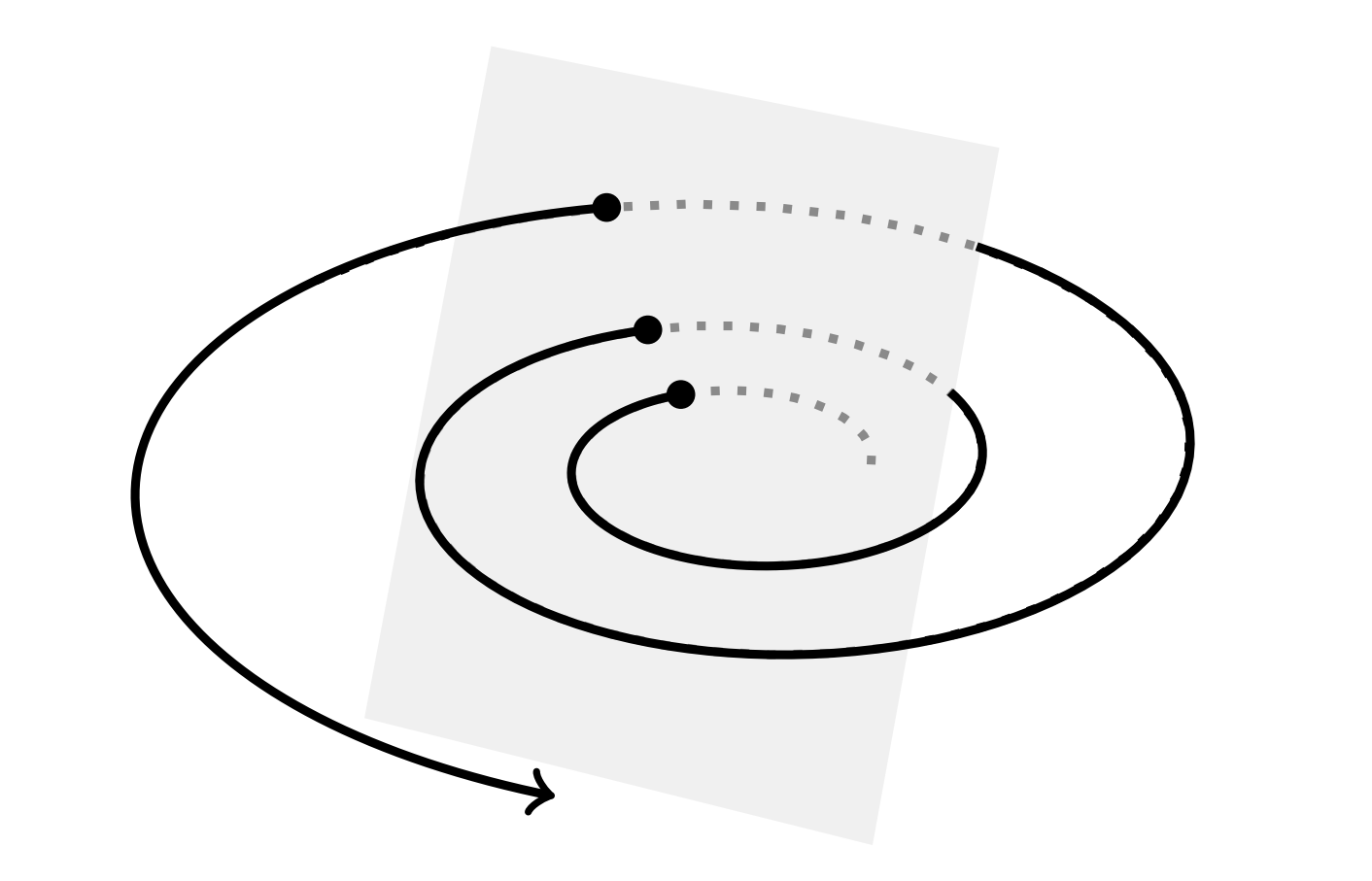
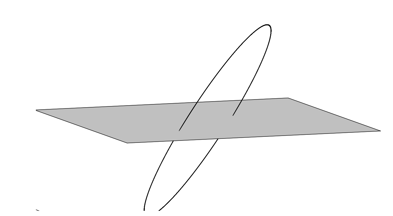
In cases for which one has periodic orbits such as the Duffing equation, Poincaré introduced the notion of surfaces of section. One embeds the orbit in a higher dimensional space so that there are no self intersections, like we saw in Figures \(\PageIndex{5}\) and \(\PageIndex{6}\). In Figure \(\PageIndex{8}\) we show an example where a simple orbit is shown as it periodically pierces a given surface.

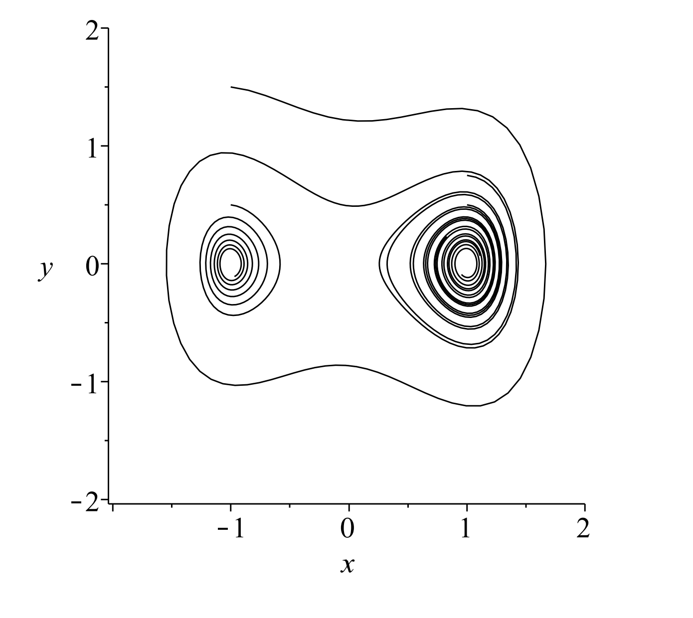
In order to simplify the resulting pictures, one only plots the points at which the orbit pierces the surface as sketched in Figure \(\PageIndex{7}\). In practice, there is a natural frequency, such as \(\omega\) in the forced Duffing equation. Then, one plots points at times that are multiples of the period, \(T=\dfrac{2 \pi}{\omega} .\) In Figure \(\PageIndex{9}\) we show what the plot for one orbit would look like for the damped, unforced Duffing equation.

Figure \(\PageIndex{4}\): Display of two orbits for the unforced Duffing equation with \(k=0.1\) and \(\Gamma=0\).

Figure \(\PageIndex{5}\): Phase plane for the Duffing equation with \(k=0.1, \Gamma=0.5\), and \(\omega=1.25\). In this case we show only one orbit which was generated from the initial condition \(\left(x_{0}=1.0, \quad y_{0}=0.5\right)\).

Figure \(\PageIndex{6}\): Phase plane for the Duffing equation with \(k=0.1, \Gamma=0.5\), and \(\omega= 1.25\). In this case four initial conditions were used to generate four orbits.

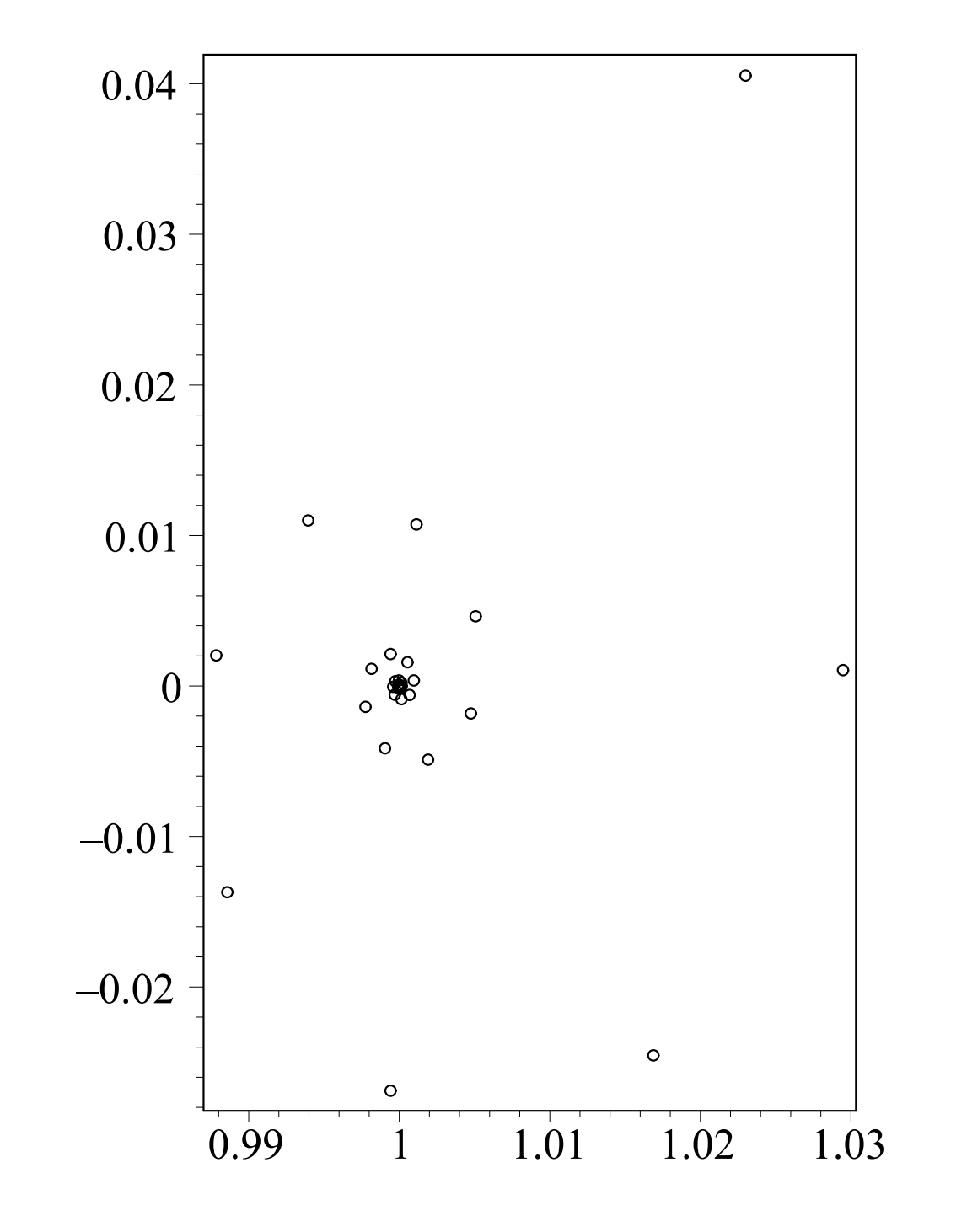
The more interesting case, is when there is forcing and damping. In this case the surface of section plot is given in Figure \(\PageIndex{10}\). While this is not as busy as the solution plot in Figure \(\PageIndex{5}\), it still provides some interesting behavior. What one finds is what is called a strange attractor. Plotting many orbits, we find that after a long time, all of the orbits are attracted to a small region in the plane, much like a stable node attracts nearby orbits. However, this set consists of more than one point. Also, the flow on the attractor is chaotic in nature. Thus, points wander in an irregular way throughout the attractor. This is one of the interesting topics in chaos theory and this whole theory of dynamical systems has only been touched in this text leaving the reader to wander of into further depth into this fascinating field.

Figure \(\PageIndex{7}\): As an orbit pierces the surface of section, one plots the point of intersection in that plane to produce the surface of section plot.

Figure \(\PageIndex{8}\): Poincaré’s surface of section. One notes each time the orbit pierces the surface.

The surface of section plots at the end of the last section were obtained using code from S. Lynch’s book Dynamical Systems with Applications Using Maple. For reference, the plots in Figures \(\PageIndex{2}\) and \(\PageIndex{3}\) were generated in Maple using the following commands:

Figure \(\PageIndex{9}\): Poincaré’s surface of section plot for the damped, unforced Duffing equation.

Figure \(\PageIndex{10}\): Poincaré’s surface of section plot for the damped, forced Duffing equation. This leads to what is known as a strange attractor.