
7.9: The Period of the Nonlinear Pendulum


- Last updated
- May 24, 2024
- Save as PDF

( \newcommand{\kernel}{\mathrm{null}\,}\)
Recall that the period of the simple pendulum is given by
for
This was based upon the solving the linear pendulum Equation 7.5.2. This equation was derived assuming a small angle approximation. How good is this approximation? What is meant by a small angle?
We recall that the Taylor series approximation of
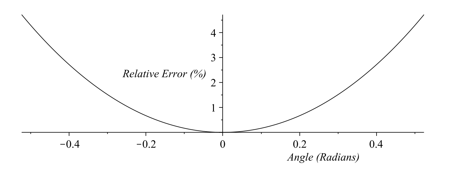
One can obtain a bound on the error when truncating this series to one term after taking a numerical analysis course. But we can just simply plot the relative error, which is defined as
A plot of the relative error is given in Figure
(Relative error in
(Solution of nonlinear pendulum equation). We next employ a technique that is useful for equations of the form
when it is easy to integrate the function
For the nonlinear pendulum problem, we multiply Equation
and note that the left side of this equation is a perfect derivative. Thus,
Therefore, the quantity in the brackets is a constant. So, we can write
Solving for
This equation is a separable first order equation and we can rearrange and integrate the terms to find that
Of course, we need to be able to do the integral. When one finds a solution in this implicit form, one says that the problem has been solved by quadratures. Namely, the solution is given in terms of some integral.
In fact, the above integral can be transformed into what is known as an elliptic integral of the first kind. We will rewrite this result and then use it to obtain an approximation to the period of oscillation of the nonlinear pendulum, leading to corrections to the linear result found earlier.
We will first rewrite the constant found in Equation
The potential energy is the gravitational potential energy. If we set the potential energy to zero at the bottom of the swing, then the potential energy is
(Total mechanical energy for the nonlinear pendulum). So, the total mechanical energy is
We note that a little rearranging shows that we can relate this result to Equation Equation
Therefore, we have determined the integration constant in terms of the total mechanical energy,
We can use Equation
Therefore, we have found that
We can solve for
Using the half angle formula,
we can rewrite the argument in the radical as
Noting that a motion from
This result can now be transformed into an elliptic integral.
and
Then, Equation
This is done by noting that
Elliptic integrals were first studied by Leonhard Euler and Giulio Carlo de’ Toschi di Fagnano
We note that the incomplete elliptic integral of the first kind is defined as
(The complete and incomplete elliptic integrals of the first kind). Then, the complete elliptic integral of the first kind is given by
Therefore, the period of the nonlinear pendulum is given by
There are table of values for elliptic integrals. However, one can use a computer algebra system to compute values of such integrals. We will look for small angle approximations.
For small angles
Inserting this expansion into the integrand for the complete elliptic integral and integrating term by term, we find that
The first term of the expansion gives the well known period of the simple pendulum for small angles. The next terms in the expression give further corrections to the linear result which are useful for larger amplitudes of oscillation. In Figure
