7.10: Exact Solutions Using Elliptic Functions
- Page ID
- 91096

THE Solution IN EQUATION 7.9.9 OF THE NONLINEAR PENDULUM EQUATION led to the introduction of elliptic integrals. The incomplete elliptic integral of the first kind is defined as
\[F(\phi, k) \equiv \int_{0}^{\phi} \dfrac{d \theta}{\sqrt{1-k^{2} \sin ^{2} \theta}}=\int_{0}^{\sin \phi} \dfrac{d z}{\sqrt{\left(1-z^{2}\right)\left(1-k^{2} z^{2}\right)}} \nonumber \]
The complete integral of the first kind is given by \(K(k)=F\left(\dfrac{\pi}{2}, k\right)\), or
\[K(k)=\int_{0}^{\pi / 2} \dfrac{d \theta}{\sqrt{1-k^{2} \sin ^{2} \theta}}=\int_{0}^{1} \dfrac{d z}{\sqrt{\left(1-z^{2}\right)\left(1-k^{2} z^{2}\right)}} \nonumber \]
Elliptic integrals of the second kind are defined as
\[E(\phi, k) =\int_{0}^{\phi} \sqrt{1-k^{2} \sin ^{2} \theta} d \theta=\int_{0}^{\sin \phi} \dfrac{\sqrt{1-k^{2} t^{2}}}{\sqrt{1-t^{2}}} d t \nonumber \]
\[E(k) =\int_{0}^{\pi / 2} \sqrt{1-k^{2} \sin ^{2} \theta} d \theta=\int_{0}^{1} \dfrac{\sqrt{1-k^{2} t^{2}}}{\sqrt{1-t^{2}}} d t \nonumber \]
Recall, a first integration of the nonlinear pendulum equation from Equation 7.9.6,
\[\left(\dfrac{d \theta}{d t}\right)^{2}-\omega^{2} \cos \theta=-\omega^{2} \cos \theta_{0} \nonumber \]
Or
\[\left(\dfrac{d \theta}{d t}\right)^{2}=2 \omega^{2}\left[\sin ^{2} \dfrac{\theta}{2}-\sin ^{2} \dfrac{\theta_{0}}{2}\right]\nonumber \]
Letting
\[k z=\sin \dfrac{\theta}{2} \text { and } k=\sin \dfrac{\theta_{0}}{2}\nonumber \]
the differential equation becomes
\[\dfrac{d z}{d \tau}=\pm \omega \sqrt{1-z^{2}} \sqrt{1-k^{2} z^{2}}\nonumber \]
Applying separation of variables, we find
\[\pm \omega\left(t-t_{0}\right) =\dfrac{1}{\omega} \int_{1}^{z} \dfrac{d z}{\sqrt{1-z^{2}} \sqrt{1-k^{2} z^{2}}} \nonumber \]
\[=\int_{0}^{1} \dfrac{d z}{\sqrt{1-z^{2}} \sqrt{1-k^{2} z^{2}}}-\int_{0}^{z} \dfrac{d z}{\sqrt{1-z^{2}} \sqrt{1-k^{2} z^{2}}} \nonumber \]
\[=K(k)-F\left(\sin ^{-1}\left(k^{-1} \sin \theta\right), k\right) \nonumber \]
The solution, \(\theta(t)\), is then found by solving for \(z\) and using \(k z=\sin \dfrac{\theta}{2}\) to solve for \(\theta\). This requires that we know how to invert the elliptic integral, \(F(z, k)\).
Elliptic functions result from the inversion of elliptic integrals. Consider
\[u(\sin \phi, k) =F(\phi, k) =\int_{0}^{\phi} \dfrac{d \theta}{\sqrt{1-k^{2} \sin ^{2} \theta}} \nonumber \]
\[=\int_{0}^{\sin \phi} \dfrac{d t}{\sqrt{\left(1-t^{2}\right)\left(1-k^{2} t^{2}\right)}} \nonumber \]
Note: \(F(\phi, 0)=\phi\) and \(F(\phi, 1)=\ln (\sec \phi+\tan \phi)\). In these cases \(F\) is obviously monotone increasing and thus there must be an inverse.
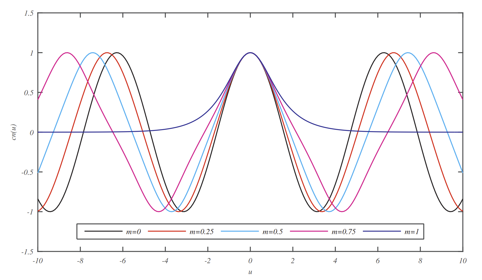
The inverse of Equation \(\PageIndex{1}\) is defined as \(\phi=F^{-1}(u, k)=\operatorname{am}(u, k)\), where \(u=\sin \phi\). The function \(\operatorname{am}(u, k)\) is called the Jacobi amplitude function and \(k\) is the elliptic modulus. [In some references and software like MATLAB packages, \(m=k^{2}\) is used as the parameter.] Three of the Jacobi elliptic functions, shown in Figure \(\PageIndex{1}\), can be defined in terms of the amplitude function by
\[\begin{aligned} &\operatorname{sn}(u, k)=\sin \operatorname{am}(u, k)=\sin \phi, \\ &\operatorname{cn}(u, k)=\cos \operatorname{am}(u, k)=\cos \phi, \end{aligned} \nonumber \]
and the delta amplitude
(Jacobi elliptic functions).
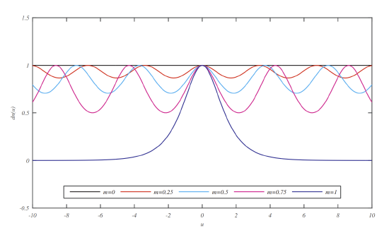
\[\operatorname{dn}(u, k)=\sqrt{1-k^{2} \sin ^{2} \phi}\nonumber. \nonumber \]
They are related through the identities
\[\mathrm{cn}^{2}(u, k)+\mathrm{sn}^{2}(u, k)=1 \nonumber \]
\[\mathrm{dn}^{2}(u, k)+k^{2} \operatorname{sn}^{2}(u, k)=1 \nonumber \]
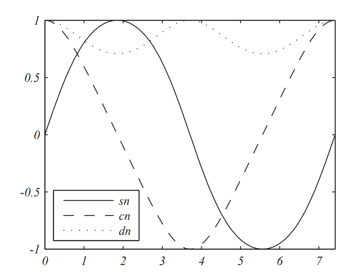
for \(m=k^{2}=0.5\). Here \(K(k)=1.8541\)
The elliptic functions can be extended to the complex plane. In this case the functions are doubly periodic. However, we will not need to consider this in the current text.
Also, we see that these functions are periodic. The period is given in rent text. terms of the complete elliptic integral of the first kind, \(K(k)\). Consider
\[ \begin{aligned} F(\phi+2 \pi, k) &=\int_{0}^{\phi+2 \pi} \dfrac{d \theta}{\sqrt{1-k^{2} \sin ^{2} \theta}} \\ &=\int_{0}^{\phi} \dfrac{d \theta}{\sqrt{1-k^{2} \sin ^{2} \theta}}+\int_{\phi}^{\phi+2 \pi} \dfrac{d \theta}{\sqrt{1-k^{2} \sin ^{2} \theta}} \\ &=F(\phi, k)+\int_{0}^{2 \pi} \dfrac{d \theta}{\sqrt{1-k^{2} \sin ^{2} \theta}} \\ &=F(\phi, k)+4 K(k) \end{aligned} \label{7.86} \]
Since \(F(\phi+2\pi , k) = u +4K\), we have
\[\operatorname{sn}(u + 4K) = \sin(\operatorname{am}(u + 4K)) = \sin(\operatorname{am}(u) + 2\pi) = \sin \operatorname{am}(u) = \operatorname{sn} u \nonumber \]
In general, we have
\[\operatorname{sn}(u+2 K, k) =-\operatorname{sn}(u, k) \nonumber \]
\[\operatorname{cn}(u+2 K, k) =-\operatorname{cn}(u, k) \nonumber \]
\[\operatorname{dn}(u+2 K, k) =\operatorname{dn}(u, k) \nonumber \]
The plots of \(\operatorname{sn}(u)\), \(\operatorname{cn}(u)\), and \(\operatorname{dn}(u)\), are shown in Figures \(\PageIndex{2}\)-\(\PageIndex{4}\).
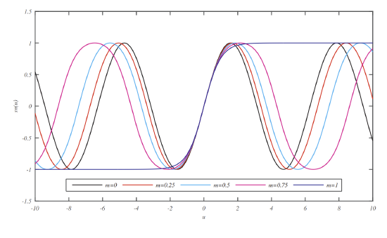
\(0,0.25,0.50,0.75,1.00\).
Namely,
\[\begin{gathered} \operatorname{sn}(u+K, k)=\dfrac{\operatorname{cn} u}{\operatorname{dn} u}, \quad \operatorname{sn}(u+2 K, k)=-\operatorname{sn} u, \\ \operatorname{cn}(u+K, k)=-\sqrt{1-k^{2} \dfrac{\operatorname{sn} u}{\operatorname{dn} u}}, \quad \operatorname{dn}(u+2 K, k)=-\operatorname{cn} u, \end{gathered} \nonumber \]
\[\operatorname{dn}(u+K, k)=\dfrac{\sqrt{1-k^{2}}}{\operatorname{dn} u}, \quad \operatorname{dn}(u+2 K, k)=\mathrm{dn} u. \nonumber \]
Therefore, dn and cn have a period of \(4 K\) and dn has a period of \(2 K\).
Special values found in Figure \(\PageIndex{1}\) are seen as
\[\begin{gathered} \operatorname{sn}(K, k)=1 \\ \operatorname{cn}(K, k)=0 \\ \operatorname{dn}(K, k)=\sqrt{1-k^{2}}=k^{\prime} \end{gathered} \nonumber \]
where \(k^{\prime}\) is called the complementary modulus.
Important to this section are the derivatives of these elliptic functions,
\[\begin{gathered} \dfrac{\partial}{\partial u} \operatorname{sn}(u, k)=\operatorname{cn}(u, k) \operatorname{dn}(u, k) \\ \dfrac{\partial}{\partial u} \operatorname{cn}(u, k)=-\operatorname{sn}(u, k) \operatorname{dn}(u, k) \\ \dfrac{\partial}{\partial u} \operatorname{dn}(u, k)=-k^{2} \operatorname{sn}(u, k) \operatorname{cn}(u, k) \end{gathered} \nonumber \]
and the amplitude function
\[\dfrac{\partial}{\partial u} \operatorname{am}(u, k)=\operatorname{dn}(u, k) \nonumber \]
Sometimes the Jacobi elliptic functions are displayed without reference to the elliptic modulus, such as \(\operatorname{sn}(u)=\operatorname{sn}(u, k)\). When \(k\) is understood, we can do the same.
Show that \(\operatorname{sn}(u)\) satisfies the differential equation
\[y^{\prime \prime}+\left(1+k^{2}\right) y=2 k^{2} y^{3} \nonumber \]
From the above derivatives, we have that
\[ \begin{aligned} \dfrac{d^{2}}{d u^{2}} \operatorname{sn}(u) &=\dfrac{d}{d u}(\operatorname{cn}(u) \operatorname{dn}(u)) \\ &=-\operatorname{sn}(u) \operatorname{dn}^{2}(u)-k^{2} \operatorname{sn}(u) \operatorname{cn}^{2}(u) \end{aligned} \label{7.90} \]
Letting \(y(u)=\operatorname{sn}(u)\) and using the identities \(\PageIndex{9}- \PageIndex{10}\), we have that
\[y^{\prime \prime}=-y\left(1-k^{2} y^{2}\right)-k^{2} y\left(1-y^{2}\right)=-\left(1+k^{2}\right) y+2 k^{2} y^{3} \nonumber \]
This is the desired result.
Show that \(\theta(t)=2 \sin ^{-1}(k \operatorname{sn} t)\) is a solution of the equation \(\ddot{\theta}+\sin \theta=0\).
Differentiating \(\theta(t)=2 \sin ^{-1}(k \operatorname{sn} t)\), we have
\[ \begin{aligned} \dfrac{d^{2}}{d t^{2}}\left(2 \sin ^{-1}(k \operatorname{sn} t)\right) &=\dfrac{d}{d t}\left(2 \dfrac{k \operatorname{cn} t \operatorname{dn} t}{\sqrt{1-k^{2} \operatorname{sn}^{2} t}}\right) \\ &=\dfrac{d}{d t}(2 k \operatorname{cn} t) \\ &=-2 k \operatorname{sn} t \operatorname{dn} t \end{aligned} \label{7.91} \]
However, we can evaluate \(\sin \theta\) for a range of \(\theta\). Thus, we have
\[ \begin{aligned} \sin \theta &=\sin \left(2 \sin ^{-1}(k \operatorname{sn} t)\right) \\ &=2 \sin \left(\sin ^{-1}(k \operatorname{sn} t)\right) \cos \left(\sin ^{-1}(k \operatorname{sn} t)\right) \\ &=2 k \operatorname{sn} t \sqrt{1-k^{2} \operatorname{sn}^{2} t} \\ &=2 k \operatorname{sn} t \operatorname{dn} t \end{aligned} \label{7.92} \]
Comparing these results, we have shown that \(\ddot{\theta}+\sin \theta=0\).
The solution to the last example can be used to obtain the exact solution to the nonlinear pendulum problem, \(\ddot{\theta}+\omega^{2} \sin \theta=0, \theta(0)=\theta_{0}, \dot{\theta}(0)=0\). The general solution is given by \(\theta(t)=2 \sin ^{-1}(k \operatorname{sn}(\omega t+\phi))\) where \(\phi\) has to be determined from the initial conditions. We note that
\[\begin{aligned} \dfrac{d \operatorname{sn}(u+K)}{d u} &=\operatorname{cn}(u+K) \operatorname{dn}(u+K) \\ &=\left(-\sqrt{1-k^{2}} \dfrac{\operatorname{sn} u}{\operatorname{dn} u}\right)\left(\dfrac{\sqrt{1-k^{2}}}{\operatorname{dn} u}\right) \\ &=-\left(1-k^{2}\right) \dfrac{\operatorname{sn} u}{\operatorname{dn}^{2} u} \end{aligned} \label{7.93} \]
Evaluating at \(u=0\), we have \(\operatorname{sn}^{\prime}(K)=0 .\)
Therefore, if we pick \(\phi=K\), then \(\dot{\theta}(0)=0\) and the solution is
\[\theta(t)=2 \sin ^{-1}(k \operatorname{sn}(\omega t+K)) \nonumber \]
Furthermore, the other initial value is found to be
\[\theta(0)=2 \sin ^{-1}(k \operatorname{sn} K)=2 \sin ^{-1} k \nonumber \]
Thus, \(k=\sin \dfrac{\theta_{0}}{2}\), as we had seen in the earlier derivation of the elliptic integral solution. The solution is given as
\[\theta(t)=2 \sin ^{-1}\left(\sin \dfrac{\theta_{0}}{2} \operatorname{sn}(\omega t+K)\right) \nonumber \]
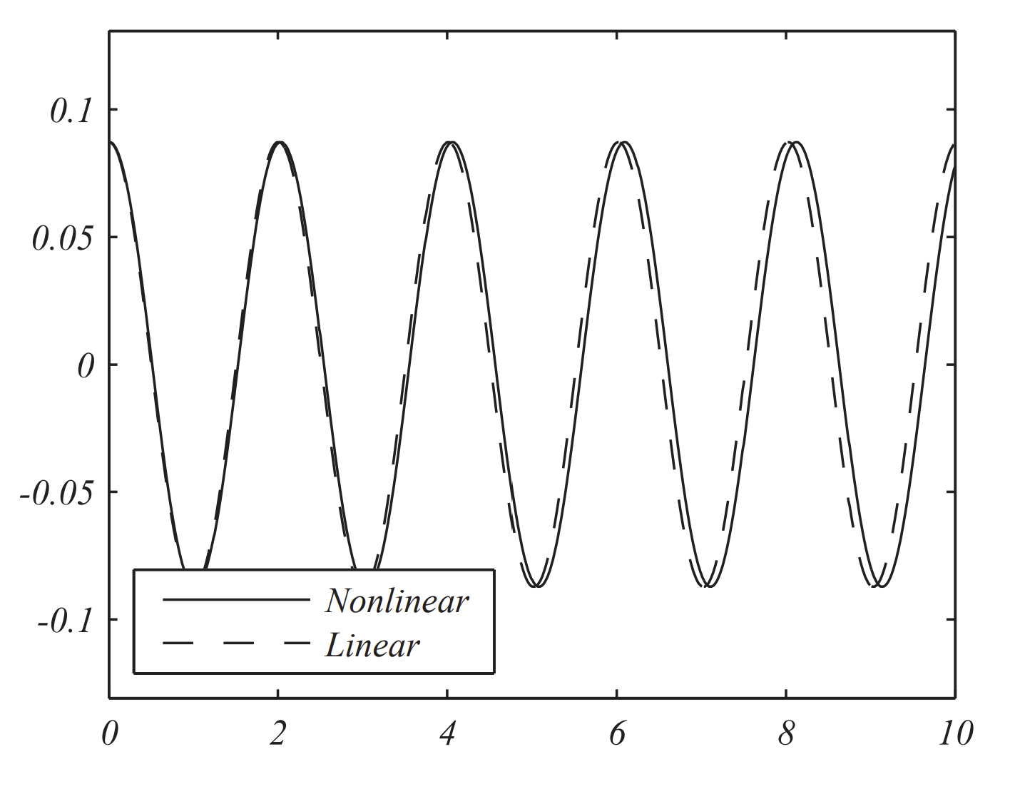
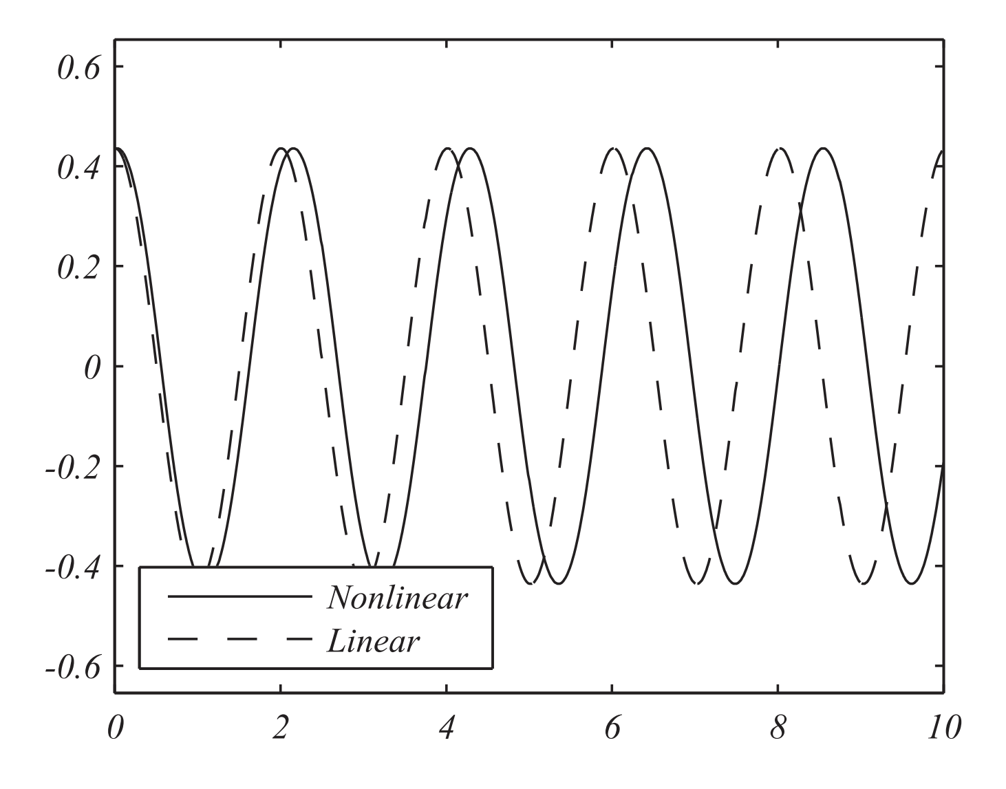
In Figures \(\PageIndex{5} - \PageIndex{6}\), we show comparisons of the exact solutions of the linear and nonlinear pendulum problems for \(L=1.0 \mathrm{~m}\) and initial angles \(\theta_{0}=10^{\circ}\) and \(\theta_{0}=50^{\circ} .\)