
7.2: The Logistic Equation


- Last updated
- May 24, 2024
- Save as PDF

( \newcommand{\kernel}{\mathrm{null}\,}\)
In this section we will explore a simple nonlinear population model. Typically, we want to model the growth of a given population, y(t), and the differential equation governing the growth behavior of this population is developed in a manner similar to that used previously for mixing problems. Namely, we note that the rate of change of the population is given by an equation of the form
dydt= Rate In − Rate Out.
The Rate In could be due to the number of births per unit time and the Rate Out by the number of deaths per unit time. While there are other potential contributions to these rates we will consider the birth and death rates in the simplest examples.
A simple population model can be obtained if one assumes that these rates are linear in the population. Thus, we assume that the
Rate In =by and the Rate Out =my.
Here we have denoted the birth rate as b and the mortality rate as m. This gives the rate of change of population as
dydt=by−my
(Malthusian population growth). Generally, these rates could depend on the time. In the case that they are both constant rates, we can define k=b−m and obtain the familiar exponential model of population growth:
dydt=ky
This is easily solved and one obtains exponential growth (k>0) or decay (k<0). This Malthusian growth model has been named after Thomas Robert Malthus (1766−1834), a clergyman who used this model to warn of the impending doom of the human race if its reproductive practices continued.
The logistic model was first published in previous exponential model takes the form 1838 by Pierre François Verhulst ( 18O4 1849) in the form
dNdt=rN(1−NK)
where N is the population at time t,r is the growth rate, and K is what is called the carrying capacity. Note that in our model r=k=Kc.
When populations get large enough, there is competition for resources, such as space and food, which can lead to a higher mortality rate. Thus, the mortality rate may be a function of the population size, m=m(y). The simplest model would be a linear dependence, m=˜m+cy. Then, the previous exponential model takes the form
dydt=ky−cy2
where k=b−˜m. This is known as the logistic model of population growth. Typically, c is small and the added nonlinear term does not really kick in until the population gets large enough.
Show that Equation 7.2.2 can be written in the form
z′=kz(1−z)
which has only one parameter.
We carry this out be rescaling the population, y(t)=αz(t), where α is to be determined. Inserting this transformation, we have
y′=ky−cy2αz′=αkz−cα2z2
Or
z′=kz(1−αckz)
Thus, we obtain the result, z′=kz(1−z), if we pick α=kc.
Before we obtain the exact solution, it is instructive to study the qualitative behavior of the solutions without actually writing down any explicit solutions. Such methods are useful for more difficult nonlinear equations as we will see later in this chapter.
We will demonstrate this analysis with a simple logistic equation example. We will first look for constant solutions, called equilibrium solutions, satisfying y′(t)=0. Then, we will look at the behavior of solutions near the equilibrium solutions, or fixed points, and determine the stability of the equilibrium solutions. In the next section we will extend these ideas to other first order differential equations.
Find and classify the equilibrium solutions of the logistic equation,
dydt=y−y2
If two solutions of the differential equation intersect then they have common values y1 at time t1. Using this information, we could set up an initial value problem for which the initial condition is y(t1)=y1. Since the two different solutions intersect at this point in the phase plane, we would have an initial value problem with two different solutions. This would violate the uniqueness theorem for initial value problems.
First, we determine the equilibrium, or constant, solutions given by y′=0. For this case, we have y−y2=0. So, the equilibrium solutions are y=0 and y=1.
These solutions divide the ty-plane into three regions, y<0,0< y<1, and y>1. Solutions that originate in one of these regions at t=t0 will remain in that region for all t>t0 since solutions of this differential equation cannot intersect.
Next, we determine the behavior of solutions in the three regions. Noting that y′(t) gives the slope of any solution in the plane, then we find that the solutions are monotonic in each region. Namely, in regions where y′(t)>0, we have monotonically increasing functions and in regions where y′(t)<0, we have monotonically decreasing functions. We determine the sign of y′(t) from the right-hand side of the differential equation.
For example, in this problem y−y2>0 only for the middle region and y−y2<0 for the other two regions. Thus, the slope is positive in the middle region, giving a rising solution as shown in Figure 7.1. Note that this solution does not cross the equilibrium solutions. Similar statements can be made about the solutions in the other regions.
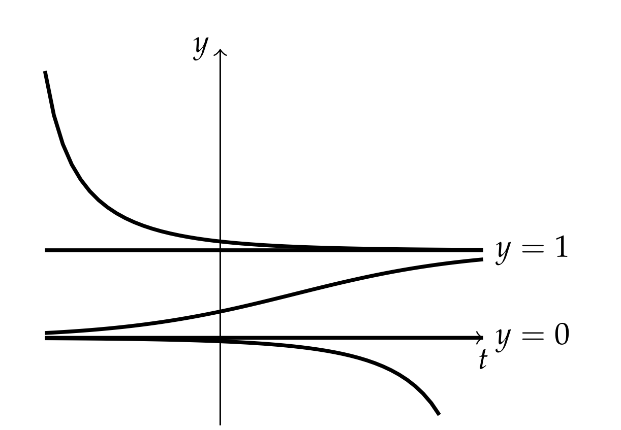
(Stable and unstable equilibria). We further note that the solutions on either side of the equilibrium solution y=1 tend to approach this equilibrium solution for large values of t. In fact, no matter how far these solutions are from y=1, as long as y(t)>0, the solutions will eventually approach this equilibrium solution as t→∞. We then say that the equilibrium solution, y=1, is a stable equilibrium.
Similarly, we note that the solutions on either side of the equilibrium solution y=0 tend away from y=0 for large values of t. No matter how close a solution is to y=0 at some given time, eventually these solutions will diverge as t→∞. We say that such equilibrium solutions are unstable equilibria.
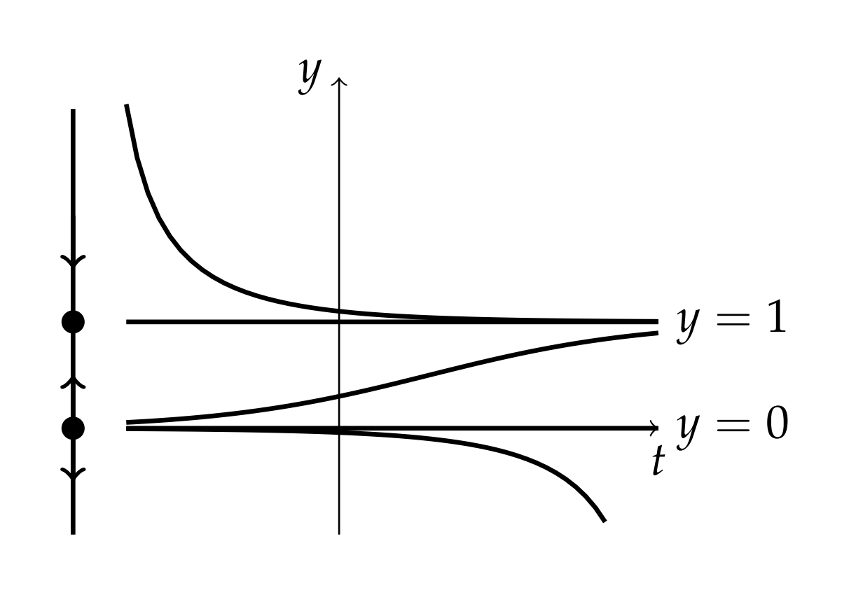
(Phase lines). If we are only interested in the behavior of the equilibrium solutions, we could just display a phase line. In Figure 7.2.2 we place a vertical line to the right of the ty-plane plot. On this line we first place dots at the corresponding equilibrium solutions and label the solutions. These points divide the phase line into three intervals.
In each interval we then place arrows pointing upward or downward indicating solutions with positive or negative slopes, respectively. For example, for the interval y>1 there is a downward pointing arrow indicating that the slope is negative in that region.
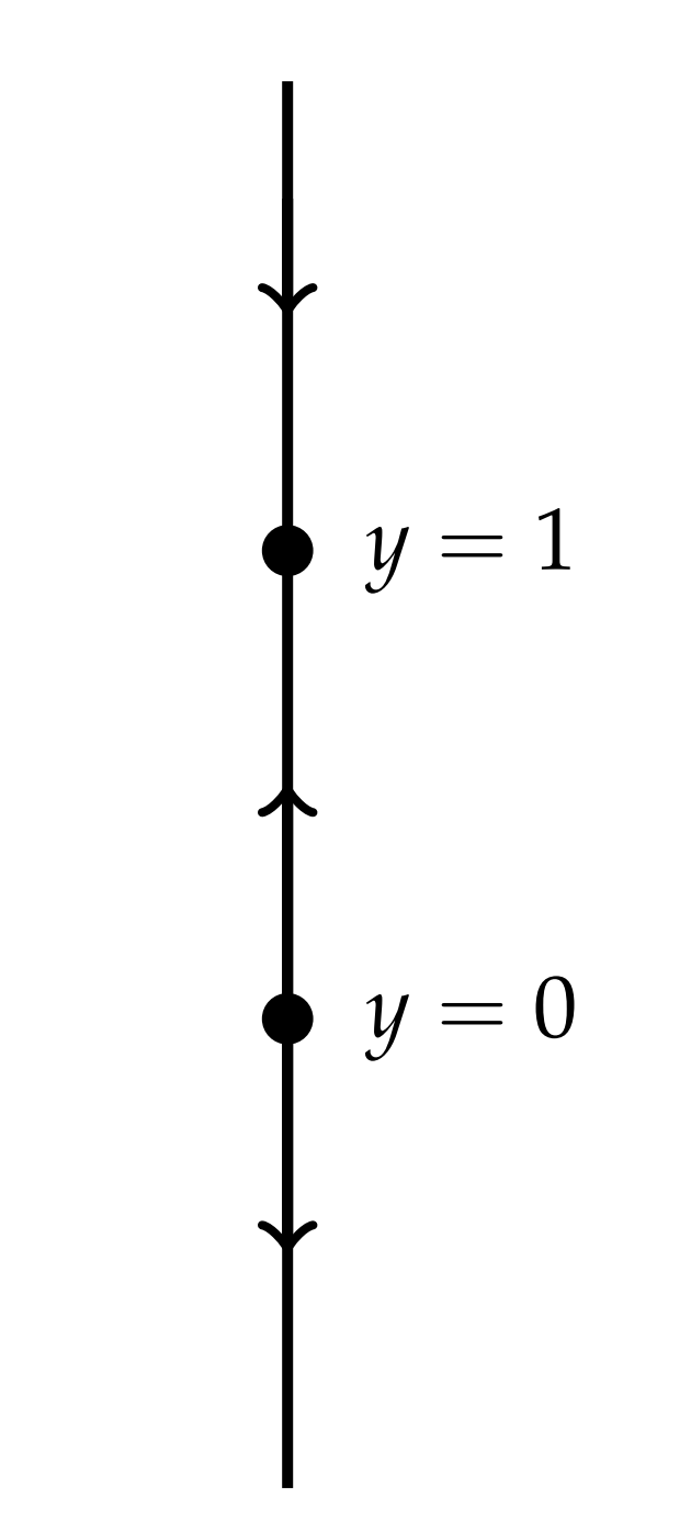
Looking at the resulting phase line we can determine if a given equilibrium is stable (arrows pointing towards the point) or unstable (arrows pointing away from the point). In Figure 7.2.3 we draw the final phase line by itself. We see that y=1 is a stable equilibrium point and y=0 is an unstable equilibrium point.
The Riccati Equation
WE HAVE SEEN THAT ONE DOES NOT NEED an explicit solution of the logistic Equation 7.2.2 in order to study the behavior of its solutions. However, the logistic equation is an example of a nonlinear first order equation that is solvable. It is also an example of a general Riccati equation, a first order differential equation quadratic in the unknown function.
The Riccati equation is named after the Italian mathematician Jacopo Francesco Riccati (1676−1754). When a(t)=0, the equation becomes a Bernoulli equation.
The general form of the Riccati equation is
dydt=a(t)+b(t)y+c(t)y2
As long as c(t)≠0, this equation can be reduced to a second order linear differential equation through the transformation
y(t)=−1c(t)x′(t)x(t).
We will demonstrate the use of this transformation in obtaining the solution of the logistic equation.
Solve the logistic equation
dydt=ky−cy2
using the transformation
y=1cx′x
differentiating this transformation with respect to t, we obtain
dydt=1c[x′′x−(x′x)2]=1c[x′′x−(cy)2]=1cx′′x−cy2
Inserting this result into the logistic equation 7.2.5, we have
1cx′′x−cy2=k1c(x′x)−cy2.
Simplifying, we see that the logistic equation has been reduced to a second order linear, differential equation,
x′′=kx′
This equation is readily solved. One integration gives
x′(t)=Bekt.
A second integration gives
x(t)=A+Bekt
where A and B are two arbitrary constants.
Inserting this result into the Riccati transformation, we obtain
y(t)=1cx′x=kBektc(A+Bekt)
It appears that we have two arbitrary constants. However, we started out with a first order differential equation and so we expect only one arbitrary constant. We can resolve this dilemma by dividing 1 the numerator and denominator by Bekt and defining C=AB. Then, we have the solution
y(t)=k/c1+Ce−kt
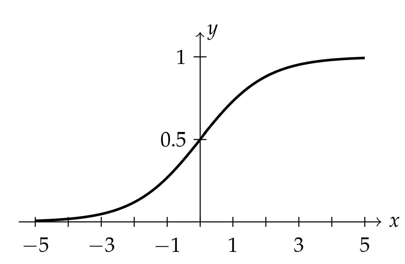
showing that there really is only one arbitrary constant in the solution. Plots of the solution 7.2.7 of the logistic equation for different initial conditions gives the solutions seen in the last section. In particular, setting all of the constants to unity, we have the sigmoid function,
y(t)=11+e−t.
This is the signature S-shaped curve of the logistic model as shown in Figure 7.2.4. We should note that this is not the only way to obtain the solution to the logistic equation, though this approach has provided us with an introduction to Riccati equations. A more direct approach would be to use separation of variables on the logistic equation, which is Problem 1.
- 1
-
This general solution holds for B≠0. If B=0, then we have x(t)=A and, thus, y(t) is the constant equilibrium solution.