1.2: The Logistic Equation
- Page ID
- 93491

\( \newcommand{\vecs}[1]{\overset { \scriptstyle \rightharpoonup} {\mathbf{#1}} } \)
\( \newcommand{\vecd}[1]{\overset{-\!-\!\rightharpoonup}{\vphantom{a}\smash {#1}}} \)
\( \newcommand{\dsum}{\displaystyle\sum\limits} \)
\( \newcommand{\dint}{\displaystyle\int\limits} \)
\( \newcommand{\dlim}{\displaystyle\lim\limits} \)
\( \newcommand{\id}{\mathrm{id}}\) \( \newcommand{\Span}{\mathrm{span}}\)
( \newcommand{\kernel}{\mathrm{null}\,}\) \( \newcommand{\range}{\mathrm{range}\,}\)
\( \newcommand{\RealPart}{\mathrm{Re}}\) \( \newcommand{\ImaginaryPart}{\mathrm{Im}}\)
\( \newcommand{\Argument}{\mathrm{Arg}}\) \( \newcommand{\norm}[1]{\| #1 \|}\)
\( \newcommand{\inner}[2]{\langle #1, #2 \rangle}\)
\( \newcommand{\Span}{\mathrm{span}}\)
\( \newcommand{\id}{\mathrm{id}}\)
\( \newcommand{\Span}{\mathrm{span}}\)
\( \newcommand{\kernel}{\mathrm{null}\,}\)
\( \newcommand{\range}{\mathrm{range}\,}\)
\( \newcommand{\RealPart}{\mathrm{Re}}\)
\( \newcommand{\ImaginaryPart}{\mathrm{Im}}\)
\( \newcommand{\Argument}{\mathrm{Arg}}\)
\( \newcommand{\norm}[1]{\| #1 \|}\)
\( \newcommand{\inner}[2]{\langle #1, #2 \rangle}\)
\( \newcommand{\Span}{\mathrm{span}}\) \( \newcommand{\AA}{\unicode[.8,0]{x212B}}\)
\( \newcommand{\vectorA}[1]{\vec{#1}} % arrow\)
\( \newcommand{\vectorAt}[1]{\vec{\text{#1}}} % arrow\)
\( \newcommand{\vectorB}[1]{\overset { \scriptstyle \rightharpoonup} {\mathbf{#1}} } \)
\( \newcommand{\vectorC}[1]{\textbf{#1}} \)
\( \newcommand{\vectorD}[1]{\overrightarrow{#1}} \)
\( \newcommand{\vectorDt}[1]{\overrightarrow{\text{#1}}} \)
\( \newcommand{\vectE}[1]{\overset{-\!-\!\rightharpoonup}{\vphantom{a}\smash{\mathbf {#1}}}} \)
\( \newcommand{\vecs}[1]{\overset { \scriptstyle \rightharpoonup} {\mathbf{#1}} } \)
\(\newcommand{\longvect}{\overrightarrow}\)
\( \newcommand{\vecd}[1]{\overset{-\!-\!\rightharpoonup}{\vphantom{a}\smash {#1}}} \)
\(\newcommand{\avec}{\mathbf a}\) \(\newcommand{\bvec}{\mathbf b}\) \(\newcommand{\cvec}{\mathbf c}\) \(\newcommand{\dvec}{\mathbf d}\) \(\newcommand{\dtil}{\widetilde{\mathbf d}}\) \(\newcommand{\evec}{\mathbf e}\) \(\newcommand{\fvec}{\mathbf f}\) \(\newcommand{\nvec}{\mathbf n}\) \(\newcommand{\pvec}{\mathbf p}\) \(\newcommand{\qvec}{\mathbf q}\) \(\newcommand{\svec}{\mathbf s}\) \(\newcommand{\tvec}{\mathbf t}\) \(\newcommand{\uvec}{\mathbf u}\) \(\newcommand{\vvec}{\mathbf v}\) \(\newcommand{\wvec}{\mathbf w}\) \(\newcommand{\xvec}{\mathbf x}\) \(\newcommand{\yvec}{\mathbf y}\) \(\newcommand{\zvec}{\mathbf z}\) \(\newcommand{\rvec}{\mathbf r}\) \(\newcommand{\mvec}{\mathbf m}\) \(\newcommand{\zerovec}{\mathbf 0}\) \(\newcommand{\onevec}{\mathbf 1}\) \(\newcommand{\real}{\mathbb R}\) \(\newcommand{\twovec}[2]{\left[\begin{array}{r}#1 \\ #2 \end{array}\right]}\) \(\newcommand{\ctwovec}[2]{\left[\begin{array}{c}#1 \\ #2 \end{array}\right]}\) \(\newcommand{\threevec}[3]{\left[\begin{array}{r}#1 \\ #2 \\ #3 \end{array}\right]}\) \(\newcommand{\cthreevec}[3]{\left[\begin{array}{c}#1 \\ #2 \\ #3 \end{array}\right]}\) \(\newcommand{\fourvec}[4]{\left[\begin{array}{r}#1 \\ #2 \\ #3 \\ #4 \end{array}\right]}\) \(\newcommand{\cfourvec}[4]{\left[\begin{array}{c}#1 \\ #2 \\ #3 \\ #4 \end{array}\right]}\) \(\newcommand{\fivevec}[5]{\left[\begin{array}{r}#1 \\ #2 \\ #3 \\ #4 \\ #5 \\ \end{array}\right]}\) \(\newcommand{\cfivevec}[5]{\left[\begin{array}{c}#1 \\ #2 \\ #3 \\ #4 \\ #5 \\ \end{array}\right]}\) \(\newcommand{\mattwo}[4]{\left[\begin{array}{rr}#1 \amp #2 \\ #3 \amp #4 \\ \end{array}\right]}\) \(\newcommand{\laspan}[1]{\text{Span}\{#1\}}\) \(\newcommand{\bcal}{\cal B}\) \(\newcommand{\ccal}{\cal C}\) \(\newcommand{\scal}{\cal S}\) \(\newcommand{\wcal}{\cal W}\) \(\newcommand{\ecal}{\cal E}\) \(\newcommand{\coords}[2]{\left\{#1\right\}_{#2}}\) \(\newcommand{\gray}[1]{\color{gray}{#1}}\) \(\newcommand{\lgray}[1]{\color{lightgray}{#1}}\) \(\newcommand{\rank}{\operatorname{rank}}\) \(\newcommand{\row}{\text{Row}}\) \(\newcommand{\col}{\text{Col}}\) \(\renewcommand{\row}{\text{Row}}\) \(\newcommand{\nul}{\text{Nul}}\) \(\newcommand{\var}{\text{Var}}\) \(\newcommand{\corr}{\text{corr}}\) \(\newcommand{\len}[1]{\left|#1\right|}\) \(\newcommand{\bbar}{\overline{\bvec}}\) \(\newcommand{\bhat}{\widehat{\bvec}}\) \(\newcommand{\bperp}{\bvec^\perp}\) \(\newcommand{\xhat}{\widehat{\xvec}}\) \(\newcommand{\vhat}{\widehat{\vvec}}\) \(\newcommand{\uhat}{\widehat{\uvec}}\) \(\newcommand{\what}{\widehat{\wvec}}\) \(\newcommand{\Sighat}{\widehat{\Sigma}}\) \(\newcommand{\lt}{<}\) \(\newcommand{\gt}{>}\) \(\newcommand{\amp}{&}\) \(\definecolor{fillinmathshade}{gray}{0.9}\)The Logistic equation
The exponential growth law for population size is unrealistic over long times. Eventually, growth will be checked by the over-consumption of resources. We assume that the environment has an intrinsic carrying capacity \(K\), and populations larger than this size experience heightened death rates.
To model population growth with an environmental carrying capacity \(K\), we look for a nonlinear equation of the form
\[\frac{d N}{d t}=r N F(N) \nonumber \]
where \(F(N)\) provides a model for environmental regulation. This function should satisfy \(F(0)=1\) (the population grows exponentially with growth rate \(r\) when \(N\) is small), \(F(K)=0\) (the population stops growing at the carrying capacity), and \(F(N)<0\) when \(N>K\) (the population decays when it is larger than the carrying capacity). The simplest function \(F(N)\) satisfying these conditions is linear and given by \(F(N)=1-N / K .\) The resulting model is the well-known logistic equation,
\[\frac{d N}{d t}=r N(1-N / K) \nonumber \]
an important model for many processes besides bounded population growth.
Although (1.2.2) is a nonlinear equation, an analytical solution can be found by separating the variables. Before we embark on this algebra, we first illustrate some basic concepts used in analyzing nonlinear differential equations.
Fixed points, also called equilibria, of a differential equation such as (1.2.2) are defined as the values of \(N\) where \(d N / d t=0\). Here, we see that the fixed points of (1.2.2) are \(N=0\) and \(N=K .\) If the initial value of \(N\) is at one of these fixed points, then \(N\) will remain fixed there for all time. Fixed points, however, can be stable or unstable. A fixed point is stable if a small perturbation from the fixed point decays to zero so that the solution returns to the fixed point. Likewise, a fixed point is unstable if a small perturbation grows exponentially so that the solution moves away from the fixed point. Calculation of stability by means of small perturbations is called linear stability analysis. For example, consider the general one-dimensional differential equation (using the notation \(\dot{x}=d x / d t\) )
\[\dot{x}=f(x) \nonumber \]
with \(x_{*}\) a fixed point of the equation, that is \(f\left(x_{*}\right)=0\). To determine analytically if \(x_{*}\) is a stable or unstable fixed point, we perturb the solution. Let us write our solution \(x=x(t)\) in the form
\[x(t)=x_{*}+\epsilon(t) \nonumber \]
where initially \(\epsilon(0)\) is small but different from zero. Substituting (1.2.4) into (1.2.3), we obtain
\[\begin{aligned} \dot{\epsilon} &=f\left(x_{*}+\epsilon\right) \\[4pt] &=f\left(x_{*}\right)+\epsilon f^{\prime}\left(x_{*}\right)+\ldots \\[4pt] &=\epsilon f^{\prime}\left(x_{*}\right)+\ldots, \end{aligned} \nonumber \]
where the second equality uses a Taylor series expansion of \(f(x)\) about \(x_{*}\) and the third equality uses \(f\left(x_{*}\right)=0\). If \(f^{\prime}\left(x_{*}\right) \neq 0\), we can neglect higher-order terms in \(\epsilon\)
for small times, and integrating we have
\[\epsilon(t)=\epsilon(0) e^{f^{\prime}\left(x_{*}\right) t} \nonumber \]
The perturbation \(\epsilon(t)\) to the fixed point \(x_{*}\) goes to zero as \(t \rightarrow \infty\) provided \(f^{\prime}\left(x_{*}\right)<\) \(0 .\) Therefore, the stability condition on \(x_{*}\) is
\[x_{*} \text { is } \begin{cases}\text { a stable fixed point if } & f^{\prime}\left(x_{*}\right)<0, \\[4pt] \text { an unstable fixed point if } & f^{\prime}\left(x_{*}\right)>0 .\end{cases} \nonumber \]
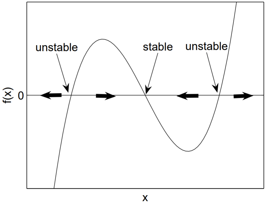
Another equivalent but sometimes simpler approach to analyzing the stability of the fixed points of a one-dimensional nonlinear equation such as (1.2.3) is to plot \(f(x)\) versus \(x\). We show a generic example in Fig. 1.1. The fixed points are the \(x\)-intercepts of the graph. Directional arrows on the \(x\)-axis can be drawn based on the sign of \(f(x)\). If \(f(x)<0\), then the arrow points to the left; if \(f(x)>0\), then the arrow points to the right. The arrows show the direction of motion for a particle at position \(x\) satisfying \(\dot{x}=f(x)\). As illustrated in Fig. 1.1, fixed points with arrows on both sides pointing in are stable, and fixed points with arrows on both sides pointing out are unstable.
In the logistic equation (1.2.2), the fixed points are \(N_{*}=0, K .\) A sketch of \(F(N)=\) \(r N(1-N / K)\) versus \(N\), with \(r, K>0\) in Fig. \(1.2\) immediately shows that \(N_{*}=0\) is an unstable fixed point and \(N_{*}=K\) is a stable fixed point. The analytical approach computes \(F^{\prime}(N)=r(1-2 N / K)\), so that \(F^{\prime}(0)=r>0\) and \(F^{\prime}(K)=-r<0\). Again we conclude that \(N_{*}=0\) is unstable and \(N_{*}=K\) is stable.
We now solve the logistic equation analytically. Although this relatively simple equation can be solved as is, we first nondimensionalize to illustrate this very important technique that will later prove to be most useful. Perhaps here one can guess the appropriate unit of time to be \(1 / r\) and the appropriate unit of population size to be \(K\). However, we prefer to demonstrate a more general technique that may be usefully applied to equations for which the appropriate dimensionless variables are difficult to guess. We begin by nondimensionalizing time and population size:
\[\tau=t / t_{*}, \quad \eta=N / N_{*} \nonumber \]
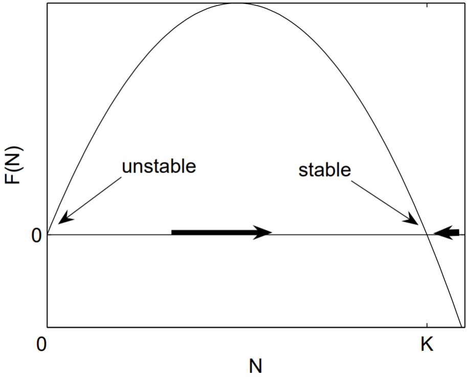
Figure 1.2: Determining stability of the fixed points of the logistic equation.
where \(t_{*}\) and \(N_{*}\) are unknown dimensional units. The derivative \(N\) is computed as
\[\frac{d N}{d t}=\frac{d\left(N_{*} \eta\right)}{d \tau} \frac{d \tau}{d t}=\frac{N_{*}}{t_{*}} \frac{d \eta}{d \tau} \nonumber \]
Therefore, the logistic equation (1.2.2) becomes
\[\frac{d \eta}{d \tau}=r t_{*} \eta\left(1-\frac{N_{*} \eta}{K}\right), \nonumber \]
which assumes the simplest form with the choices \(t_{*}=1 / r\) and \(N_{*}=K\). Therefore, our dimensionless variables are
\[\tau=r t, \quad \eta=N / K \nonumber \]
and the logistic equation, in dimensionless form, becomes
\[\frac{d \eta}{d \tau}=\eta(1-\eta) \text {, } \nonumber \]
with the dimensionless initial condition \(\eta(0)=\eta_{0}=N_{0} / K\), where \(N_{0}\) is the initial population size. Note that the dimensionless logistic equation (1.4) has no free parameters, while the dimensional form of the equation (1.2.2) contains \(r\) and \(K\). Reduction in the number of free parameters (here, two: \(r\) and \(K\) ) by the number of independent units (here, also two: time and population size) is a general feature of nondimensionalization. The theoretical result is known as the Buckingham Pi Theorem. Reducing the number of free parameters in a problem to the absolute minimum is especially important before proceeding to a numerical solution. The parameter space that must be explored may be substantially reduced.
Solving the dimensionless logistic equation (1.4) can proceed by separating the variables. Separating and integrating from \(\tau=0\) to \(\tau\) and \(\eta_{0}\) to \(\eta\) yields
\[\int_{\eta_{0}}^{\eta} \frac{d \eta}{\eta(1-\eta)}=\int_{0}^{\tau} d \tau \nonumber \]
The integral on the left-hand-side can be performed using the method of partial fractions:
\[\begin{aligned} \frac{1}{\eta(1-\eta)} &=\frac{A}{\eta}+\frac{B}{1-\eta} \\[4pt] &=\frac{A+(B-A) \eta}{\eta(1-\eta)} \end{aligned} \nonumber \]
and by equating the coefficients of the numerators proportional to \(\eta^{0}\) and \(\eta^{1}\), we find that \(A=1\) and \(B=1\). Therefore,
\[\begin{aligned} \int_{\eta_{0}}^{\eta} \frac{d \eta}{\eta(1-\eta)} &=\int_{\eta_{0}}^{\eta} \frac{d \eta}{\eta}+\int_{\eta_{0}}^{\eta} \frac{d \eta}{(1-\eta)} \\[4pt] &=\ln \frac{\eta}{\eta_{0}}-\ln \frac{1-\eta}{1-\eta_{0}} \\[4pt] &=\ln \frac{\eta\left(1-\eta_{0}\right)}{\eta_{0}(1-\eta)} \\[4pt] &=\tau \end{aligned} \nonumber \]
Solving for \(\eta\), we first exponentiate both sides and then isolate \(\eta:\)
\[\begin{aligned} &\frac{\eta\left(1-\eta_{0}\right)}{\eta_{0}(1-\eta)}=e^{\tau}, \text { or } \quad \eta\left(1-\eta_{0}\right)=\eta_{0} e^{\tau}-\eta \eta_{0} e^{\tau} \\[4pt] &\text { or } \eta\left(1-\eta_{0}+\eta_{0} e^{\tau}\right)=\eta_{0} e^{\tau}, \text { or } \quad \eta=\frac{\eta_{0}}{\eta_{0}+\left(1-\eta_{0}\right) e^{-\tau}} \end{aligned} \nonumber \]
Returning to the dimensional variables, we finally have
\[N(t)=\frac{N_{0}}{N_{0} / K+\left(1-N_{0} / K\right) e^{-r t}} \nonumber \]
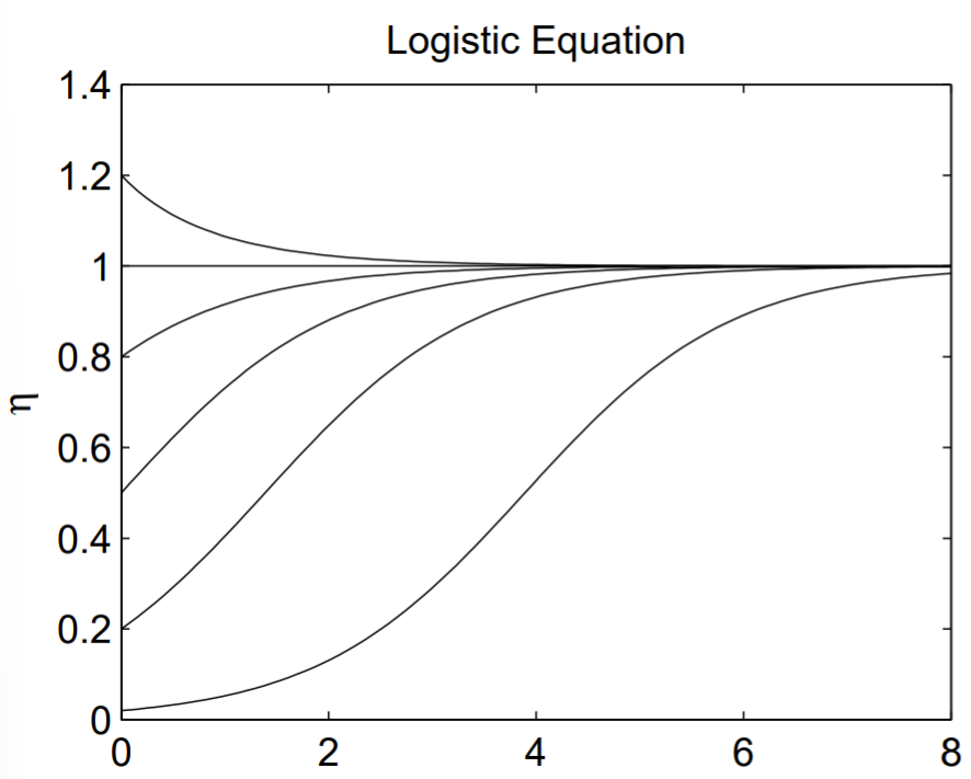
There are several ways to write the final result given by (1.5). The presentation of a mathematical result requires a good aesthetic sense and is an important element of mathematical technique. When deciding how to write (1.5), I considered if it was easy to observe the following limiting results: (1) \(N(0)=N_{0} ;(2) \lim _{t \rightarrow \infty} N(t)=K\); and (3) \(\lim _{K \rightarrow \infty} N(t)=N_{0} \exp (r t)\)
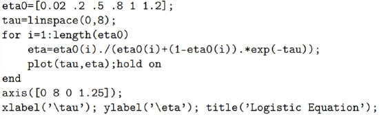
In Fig. 1.3, we plot the solution to the dimensionless logistic equation for initial conditions \(\eta_{0}=0.02,0.2,0.5,0.8,1.0\), and \(1.2\). The lowest curve is the characteristic ’S-shape’ usually associated with the solution of the logistic equation. This sigmoidal curve appears in many other types of models. The MATLAB script to produce Fig. \(1.3\) is shown below.