7.5: The Stability of Fixed Points in Nonlinear Systems

We next investigate the stability of the equilibrium solutions of the nonlinear pendulum which we first encountered in section 2.3.2 . Along the way we will develop some basic methods for studying the stability of equilibria in nonlinear systems in general.

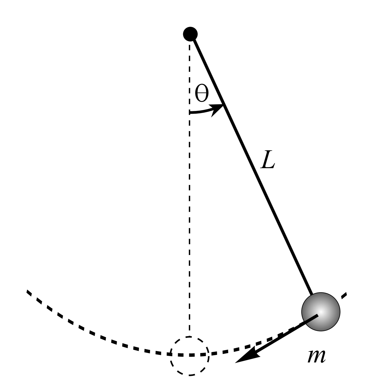
Recall that the derivation of the pendulum equation was based upon a simple point mass \(m\) hanging on a string of length \(L\) from some support as shown in Figure \(\PageIndex{1}\). One pulls the mass back to some starting angle, \(\theta_{0}\), and releases it. The goal is to find the angular position as a function of time, \(\theta(t)\).

In Chapter 2 we derived the nonlinear pendulum equation,

\[L \ddot{\theta}+g \sin \theta=0 \nonumber \]

There are several variations of Equation \(\PageIndex{1}\) which we have used in this text. The first one is the linear pendulum, which was obtained using a small angle approximation,

\[L \ddot{\theta}+g \theta=0 \nonumber \]

Figure \(\PageIndex{1}\): A simple pendulum consists of a point mass \(m\) attached to a string of length \(L\). It is released from an angle \(\theta_0\).

We also made the system more realistic by adding damping and forcing. A variety of these oscillation problems are summarized in the table below.

Equations for Pendulum Motion

1. Nonlinear Pendulum: \(L \ddot{\theta}+g \sin \theta=0\).
2. Damped Nonlinear Pendulum: \(L \ddot{\theta}+b \dot{\theta}+g \sin \theta=0\).
3. Linear Pendulum: \(L \ddot{\theta}+g \theta=0\).
4. Damped Linear Pendulum: \(L \ddot{\theta}+b \dot{\theta}+g \theta=0\).
5. Forced Damped Nonlinear Pendulum: \(L \ddot{\theta}+b \dot{\theta}+g \sin \theta=F \cos \omega t\).
6. Forced Damped Linear Pendulum: \(L \ddot{\theta}+b \dot{\theta}+g \theta=F \cos \omega t\).

There are two simple systems that we will consider, the damped linear pendulum, in the form

\[x^{\prime \prime}+b x^{\prime}+\omega^{2} x=0 \nonumber \]

and the the damped nonlinear pendulum, in the form

\[x^{\prime \prime}+b x^{\prime}+\omega^{2} \sin x=0 \nonumber \]

These are second order differential equations and can be cast as a system of two first order differential equations using the methods of Chapter \(6 \).

The linear equation can be written as

\[ \begin{aligned} &x^{\prime}=y \\[4pt] &y^{\prime}=-b y-\omega^{2} x \end{aligned} \label{7.13} \]

This system has only one equilibrium solution, \(x=0, y=0\).

The damped nonlinear pendulum takes the form

\[ \begin{aligned} x^{\prime} &=y \\[4pt] y^{\prime} &=-b y-\omega^{2} \sin x \end{aligned} \label{7.14} \]

This system also has the equilibrium solution \(x=0, y=0\). However, there are actually an infinite number of solutions. The equilibria are determined from

\[y=0 \text { and }-b y-\omega^{2} \sin x=0 \nonumber \]

These equations imply that \(y=0\) and \(\sin x=0\). There are an infinite number of solutions to the latter equation: \(x=n \pi, n=0, \pm 1, \pm 2, \ldots\). So, this system has an infinite number of equilibria, \((n \pi, 0), n=0, \pm 1, \pm 2, \ldots\)

The next step is to determine the stability of the equilibrium solutions these systems. This can be accomplished just as we had done for first order equations. To do this we need a more general theory for nonlinear systems. So, we will develop the needed machinery.

We begin with the \(n\)-dimensional system

\[\mathbf{x}^{\prime}=\mathbf{f}(\mathbf{x}), \quad \mathbf{x} \in \mathrm{R}^{n} \nonumber \]

Here \(\mathbf{f}: \mathrm{R}^{n} \rightarrow \mathrm{R}^{n}\) is a mapping from \(\mathrm{R}^{n}\) to \(\mathrm{R}^{n}\). We define the equilibrium solutions, or fixed points, of this system as the points \(\mathbf{x}^{*}\) satisfying \(f(x^{*}) =0\).

Figure \(\PageIndex{2}\): A general point in the plane, which is near the fixed point, in the form \(\mathbf{x}=\mathbf{x}^{*}+\xi\)

(Linear stability analysis of systems). The stability in the neighborhood of equilibria will now be determined. We are interested in what happens to solutions of the system with initial conditions starting near a fixed point. We will represent a general point in the plane, which is near the fixed point, in the form \(\mathbf{x}=\mathbf{x}^{*}+\xi\). We note that the length of \(\xi\) gives an indication of how close we are to the fixed point. So, we consider that initially, \(|\xi| \ll 1\).

As the system evolves, \(\xi\) will change. The change of \(\xi\) in time is in turn governed by a system of equations. We can approximate this evolution as follows. First, we note that

\[\mathbf{x}^{\prime}=\xi^{\prime}\nonumber \]

Next, we have that

\[\mathbf{x}=\mathbf{x}^{*}+\xi\nonumber \]

We can expand the right side about the fixed point using a multidimensional version of Taylor’s Theorem. Thus, we have that

\[\mathbf{f}\left(\mathbf{x}^{*}+\xi\right)=\mathbf{f}\left(\mathbf{x}^{*}\right)+D \mathbf{f}\left(\mathbf{x}^{*}\right) \xi+O\left(|\xi|^{2}\right) \nonumber \]

(The Jacobian matrix). Here \(D \mathbf{f}(\mathbf{x})\) is the Jacobian matrix, defined as

\[D \mathbf{f}\left(\mathbf{x}^{*}\right) \equiv\left(\begin{array}{cccc} \dfrac{\partial f_{1}}{\partial x_{1}} & \dfrac{\partial f_{1}}{\partial x_{2}} & \cdots & \dfrac{\partial f_{1}}{\partial x_{n}} \\[4pt] \dfrac{\partial f_{2}}{\partial x_{1}} & \ddots & \ddots & \vdots \\[4pt] \vdots & \ddots & \ddots & \vdots \\[4pt] \dfrac{\partial f_{n}}{\partial x_{1}} & \cdots & \cdots & \dfrac{\partial f_{n}}{\partial x_{n}} \end{array}\right) \nonumber. \nonumber \]

Noting that \(\mathbf{f}\left(\mathbf{x}^{*}\right)=\mathbf{0}\), we then have that System \(\PageIndex{6}\) becomes

\[\xi^{\prime} \approx D \mathbf{f}\left(\mathbf{x}^{*}\right) \xi \nonumber \]

It is this equation which describes the behavior of the system near the fixed point. As with first order equations, we say that System \(\PageIndex{6}\) has been linearized or that Equation \(\PageIndex{7}\) is the linearization of System \(\PageIndex{6}\).

(Linearization of the system \(\mathbf{x}^{\prime}=\mathbf{f}(\mathbf{x})\)). The stability of the equilibrium point of the nonlinear system is now reduced to analyzing the behavior of the linearized system given by Equation \(\PageIndex{7}\). We can use the methods from the last two chapters to investigate the eigenvalues of the Jacobian matrix evaluated at each equilibrium point. We will demonstrate this procedure with several examples.

Example \(\PageIndex{1}\)

Determine the equilibrium points and their stability for the system

\[ \begin{aligned} &x^{\prime}=-2 x-3 x y \\[4pt] &y^{\prime}=3 y-y^{2} \end{aligned} \label{7.18} \]

We first determine the fixed points. Setting the right-hand side equal to zero and factoring, we have

\[ \begin{aligned} -x(2+3 y) &=0 \\[4pt] y(3-y) &=0 \end{aligned} \label{7.19} \]

From the second equation, we see that either \(y=0\) or \(y=3 \). The first equation then gives \(x=0\) in either case. So, there are two fixed points: \((0,0)\) and \((0,3)\).

Next, we linearize the system of differential equations about each fixed point. First, we note that the Jacobian matrix is given by

\[D \mathbf{f}(x, y)=\left(\begin{array}{cc} -2-3 y & -3 x \\[4pt] 0 & 3-2 y \end{array}\right) \nonumber \]

1. Case I Equilibrium point \((0,0)\).

In this case we find that

\[D \mathbf{f}(0,0)=\left(\begin{array}{cc} -2 & 0 \\[4pt] 0 & 3 \end{array}\right) \nonumber \]

Therefore, the linearized equation becomes

\[\xi^{\prime}=\left(\begin{array}{cc} -2 & 0 \\[4pt] 0 & 3 \end{array}\right) \xi \nonumber \]

This is equivalently written out as the system

\[ \begin{aligned} &\xi_{1}^{\prime}=-2 \xi_{1} \\[4pt] &\xi_{2}^{\prime}=3 \xi_{2} . \end{aligned} \label{7.23} \]

This is the linearized system about the origin. Note the similarity with the original system. We should emphasize that the linearized equations are constant coefficient equations and we can use matrix methods to determine the nature of the equilibrium point. The eigenvalues of this system are obviously \(\lambda=-2,3\). Therefore, we have that the origin is a saddle point.

2. Case II Equilibrium point \((0,3)\).

Again we evaluate the Jacobian matrix at the equilibrium point and look at its eigenvalues to determine the type of fixed point. The Jacobian matrix for this case becomes

\[D \mathbf{f}(0,3)=\left(\begin{array}{cc} -11 & 0 \\[4pt] 0 & -3 \end{array}\right) \nonumber \]

The eigenvalues are \(\lambda=-11,-3 \). So, this fixed point is a stable node.

Figure \(\PageIndex{3}\): Phase plane for the system \(x^{\prime}=-2 x-3 x y, y^{\prime}=3 y-y^{2} \).

This analysis has given us a saddle and a stable node. We know what the behavior is like near each fixed point, but we have to resort to other means to say anything about the behavior far from these points. The phase portrait for this system is given in Figure \(\PageIndex{3}\). You should be able to locate the saddle point and the node in the figure. Notice how solutions behave in regions far from these points.

We can expect to be able to perform a linearization under general conditions. These are given in the Hartman-Grofman Theorem:

Theorem \(\PageIndex{1}\)

A continuous map exists between the linear and nonlinear systems when \(D \mathbf{f}\left(\mathbf{x}^{*}\right)\) does not have any eigenvalues with zero real part.

Generally, there are several types of behavior that one can see in nonlinear systems. One can see sinks or sources, hyperbolic (saddle) points, elliptic points (centers) or foci. We have defined some of these for planar systems. In general, if at least two eigenvalues have real parts with opposite signs, then the fixed point is a hyperbolic point. If the real part of a nonzero eigenvalue is zero, then we have a center, or elliptic point.

For linear systems in the plane, this classification was done in Chapter 6 . The Jacobian matrix evaluated at the equilibrium points is simply the \(2 \times 2\) coefficient matrix we had called \(A\).

\[J=\left(\begin{array}{ll} a & b \\[4pt] c & d \end{array}\right) \text {. } \nonumber \]

Here we are using \(J=D \mathbf{f}\left(\mathbf{x}^{*}\right)\).

The eigenvalue equation is given by

\[\lambda^{2}-(a+d) \lambda+(a d-b c)=0 \nonumber \]

However, \(a+d\) is the trace, \(\operatorname{tr}(J)\) and \(\operatorname{det}(J)=a d-b c\). Therefore, we can write the eigenvalue equation as

\[\lambda^{2}-\operatorname{tr}(J) \lambda+\operatorname{det}(J)=0 \nonumber \]

The solution of this equation is found using the quadratic formula,

\[\lambda=\dfrac{1}{2}\left[-\operatorname{tr}(J) \pm \sqrt{\operatorname{tr}^{2}(J)-4 \operatorname{det}(J)}\right]\nonumber \]

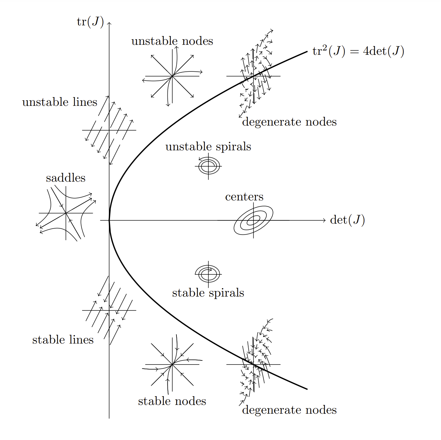
We had seen in previous chapter that equilibrium points in planar systems can be classified as nodes, saddles, centers, or spirals (foci). The type of behavior can be determined from solutions of the eigenvalue equation. Since the nature of the eigenvalues depends on the trace and determinant of the Jacobian matrix at the equilibrium point, we can relate the types of equilibria to points in the det-tr plane. This is shown in Figure \(\PageIndex{4}\), which is similar to Figure 6.7.1.

In Figure \(\PageIndex{4}\) the parabola \(\operatorname{tr}^{2}(J)=4 \operatorname{det}(J)\) divides the det-tr plane. Points on this curve give a vanishing discriminant in the computation of the eigenvalues. In these cases one finds repeated roots, or eigenvalues. Along this curve one can find stable and unstable degenerate nodes. Also along this line are stable and unstable proper nodes, called star nodes. These arise from systems of the form \(x^{\prime}=a x, y^{\prime}=a y\).

In the case that \(\operatorname{det}(J)<0\), we have that the discriminant

\[\Delta \equiv \operatorname{tr}^{2}(J)-4 \operatorname{det}(J)\nonumber \]

is positive. Not only that, \(\Delta>\operatorname{tr}^{2}(J)\). Thus, we obtain two real and distinct eigenvalues with opposite signs. These lead to saddle points.

In the case that \(\operatorname{det}(J)>0\), we can have either \(\Delta>0\) or \(\Delta<0 \). The discriminant is negative for points inside the parabolic curve. It is in this region that one finds centers and spirals, corresponding to complex eigenvalues. When \(\operatorname{tr}(J)>0\), there are unstable spirals. There are stable spirals when \(\operatorname{tr}(J)<0\). For the case that \(\operatorname{tr}(J)=0\), the eigenvalues are pure imaginary, giving centers.

There are several other types of behavior depicted in the figure, but we will now turn to studying a few of examples.

Figure \(\PageIndex{4}\): Diagram indicating the behavior of equilibrium points in the det tr plane. The parabolic curve

\[\operatorname{tr}^{2}(J)=4 \operatorname{det}(J) \nonumber \]

indicates where the discriminant vanishes.

Example \(\PageIndex{2}\)

Find and classify all the equilibrium solutions of the nonlinear system.

\[ \begin{aligned} &x^{\prime}=2 x-y+2 x y+3\left(x^{2}-y^{2}\right) \\[4pt] &y^{\prime}=x-3 y+x y-3\left(x^{2}-y^{2}\right) \end{aligned}\label{7.26} \]

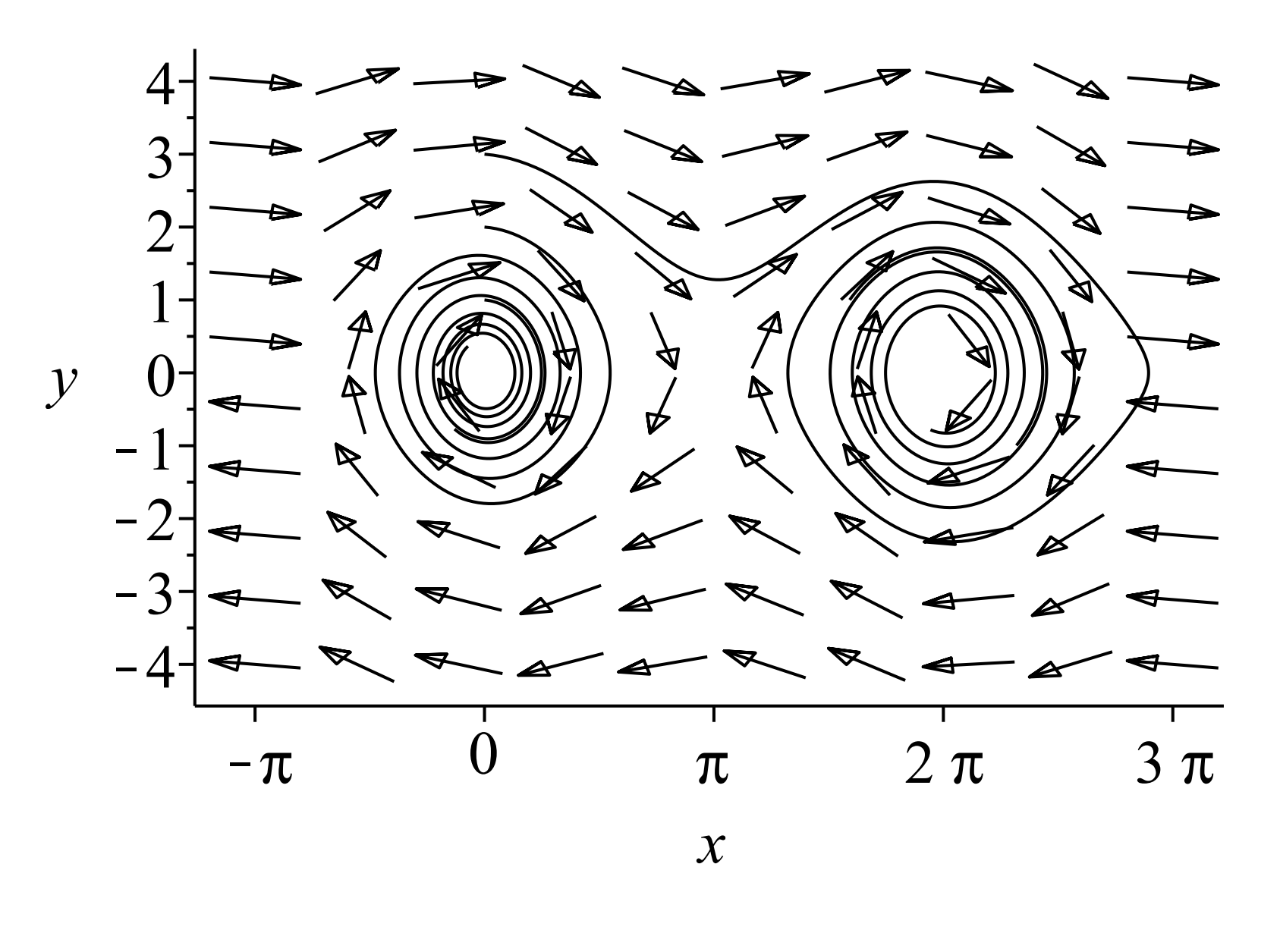
In Figure \(\PageIndex{5}\) we show the direction field for this system. Try to locate and classify the equilibrium points visually. After the stability analysis, you should return to this figure and determine if you identified the equilibrium points correctly.

We will first determine the equilibrium points. Setting the righthand side of each differential equation to zero, we have

\[ \begin{aligned} 2 x-y+2 x y+3\left(x^{2}-y^{2}\right) &=0 \\[4pt] x-3 y+x y-3\left(x^{2}-y^{2}\right) &=0 \end{aligned} \label{7.27} \]

This system of algebraic equations can be solved exactly. Adding the equations, we have

\[3 x-4 y+3 x y=0 \nonumber \]

Figure \(\PageIndex{5}\): Phase plane for the system

\[\begin{aligned} &x^{\prime}=2 x-y+2 x y+3\left(x^{2}-y^{2}\right), \\[4pt] &y^{\prime}=x-3 y+x y-3\left(x^{2}-y^{2}\right) . \end{aligned} \nonumber \]

Solving for \(x\),

\[x=\dfrac{4 y}{3(1+y)} \nonumber \]

and substituting the result for \(x\) into the first algebraic equation, we find an equation for \(y\) :

\[\dfrac{y(1-y)\left(9 y^{2}+22 y+5\right)}{3(1+y)^{2}}=0.\nonumber \]

The solutions to this equation are

\[y=0,1,-\dfrac{11}{9} \pm \dfrac{2}{9} \sqrt{19}\nonumber \]

The corresponding values for \(x\) are

\[x=0, \dfrac{2}{3}, 1 \mp \dfrac{\sqrt{19}}{3}.\nonumber \]

Now that we have located the equilibria, we can classify them. The Jacobian matrix is given by

\[D \mathbf{f}(x, y)=\left(\begin{array}{cc} 6 x+2 y+2 & 2 x-6 y-1 \\[4pt] -6 x+y+1 & x+6 y-3 \end{array}\right) \nonumber \]

Now, we evaluate the Jacobian at each equilibrium point and find the eigenvalues.

1. Case I. Equilibrium point \((0,0)\).

In this case we find that

\[D \mathbf{f}(0,0)=\left(\begin{array}{cc} -2 & -1 \\[4pt] 1 & -3 \end{array}\right) \nonumber \]

The eigenvalues of this matrix are \(\lambda=-\dfrac{1}{2} \pm \dfrac{\sqrt{21}}{2} \). Therefore, the origin is a saddle point.

2. Case II. Equilibrium point \(\left(\dfrac{2}{3}, 1\right)\).

Again we evaluate the Jacobian matrix at the equilibrium point and look at its eigenvalues to determine the type of fixed point. The Jacobian matrix for this case becomes

\[D f\left(\dfrac{2}{3}, 1\right)=\left(\begin{array}{cc} 8 & -\dfrac{17}{3} \\[4pt] -2 & \dfrac{11}{3} \end{array}\right) \nonumber \]

The eigenvalues are \(\lambda=\dfrac{35}{6} \pm \dfrac{\sqrt{577}}{6} \approx 9.84,1.83 \). This fixed point is an unstable node.

3. Case III. Equilibrium point \(\left(1 \mp \dfrac{\sqrt{19}}{3},-\dfrac{11}{9} \pm \dfrac{2}{9} \sqrt{19}\right)\).

The Jacobian matrix for this case becomes

\[D f\left(1 \mp \dfrac{\sqrt{19}}{3},-\dfrac{11}{9} \pm \dfrac{2}{9} \sqrt{19}\right)=\left(\begin{array}{cc} \dfrac{50}{9} \mp \dfrac{14}{9} \sqrt{19} & \dfrac{25}{3} \mp 2 \sqrt{19} \\[4pt] -\dfrac{56}{9} \pm \dfrac{20}{9} \sqrt{19} & -\dfrac{28}{3} \pm \sqrt{19} \end{array}\right) \nonumber \]

There are two equilibrium points under this case. The first is given by

\[\left(1-\dfrac{\sqrt{19}}{3},-\dfrac{11}{9}+\dfrac{2}{9} \sqrt{19}\right) \approx(0.453,-0.254)\nonumber \]

The eigenvalues for this point are

\[\lambda=-\dfrac{17}{9}-\dfrac{5}{18} \sqrt{19} \pm \dfrac{1}{18} \sqrt{3868 \sqrt{19}-16153}\nonumber \]

These are approximately \(-4.58\) and \(-1.62\) So, this equilibrium point is a stable node.

The other equilibrium is \(\left(1+\dfrac{\sqrt{19}}{3},-\dfrac{11}{9}-\dfrac{2}{9} \sqrt{19}\right) \approx(2.45,-2.19) \). The corresponding eigenvalues are complex with negative real parts,

\[\lambda=-\dfrac{17}{9}+\dfrac{5}{18} \sqrt{19} \pm \dfrac{i}{18} \sqrt{16153+3868 \sqrt{19}}\nonumber \]

or \(\lambda \approx-0.678 \pm 10.1 i\). This point is a stable spiral.

Plots of the phase plane are given in Figures \(\PageIndex{3}\) and \(\PageIndex{5}\). The reader can look at the direction field and verify these results for the behavior of equilibrium solutions. A zoomed in view is shown in Figure \(\PageIndex{6}\) with several orbits indicated.

Figure \(\PageIndex{6}\): A closer look at the phase plane for the system

\[\begin{gathered} x^{\prime}=2 x-y+2 x y+3\left(x^{2}-y^{2}\right) \\[4pt] y^{\prime}=x-3 y+x y-3\left(x^{2}-y^{2}\right) \end{gathered}\nonumber \]

with a few trajectories shown.

Example \(\PageIndex{3}\)Damped Nonlinear Pendulum Equilibria

We are now ready to establish the behavior of the fixed points of the damped nonlinear pendulum system in Equation \(\PageIndex{4}\). Recall that the system for the damped nonlinear pendulum was given by

\[ \begin{aligned} x^{\prime} &=y \\[4pt] y^{\prime} &=-b y-\omega^{2} \sin x \end{aligned} \label{7.32} \]

For a damped system, we will need \(b>0\). We had found that there are an infinite number of equilibrium points at \((n \pi, 0), n=0, \pm 1, \pm 2, \ldots\)

The Jacobian matrix for this systems is

\[ D \mathbf{f}(x, y)=\left(\begin{array}{cc} 0 & 1 \\[4pt] -\omega^{2} \cos x & -b \end{array}\right) \nonumber \]

Evaluating this matrix at the fixed points, we find that

\[D \mathbf{f}(n \pi, 0)=\left(\begin{array}{cc}0 & 1 \\[4pt] -\omega^{2} \cos n \pi & -b\end{array}\right)=\left(\begin{array}{cc}0 & 1 \\[4pt] (-1)^{n+1} \omega^{2} & -b\end{array}\right) \nonumber \]

The eigenvalue equation is given by

\[\lambda^{2}+b \lambda+(-1)^{n} \omega^{2}=0 \nonumber \]

There are two cases to consider: \(n\) even and \(n\) odd. For the first case, we find the eigenvalues

\[\lambda=\dfrac{-b \pm \sqrt{b^{2}-4 \omega^{2}}}{2} \nonumber \]

For \(b^{2}<4 \omega^{2}\), we have two complex conjugate roots with a negative real part. Thus, we have stable foci for even \(n\) values. If there is no damping, then we obtain centers \((\lambda=\pm i \omega)\).

In the second case, \(n\) odd, we find

\[\lambda=\dfrac{-b \pm \sqrt{b^{2}+4 \omega^{2}}}{2} \nonumber \]

Since \(b^{2}+4 \omega^{2}>b^{2}\), these roots will be real with opposite signs. Thus, we have hyperbolic points, or saddles. If there is no damping, the eigenvalues reduce to \(\lambda=\pm \omega\).

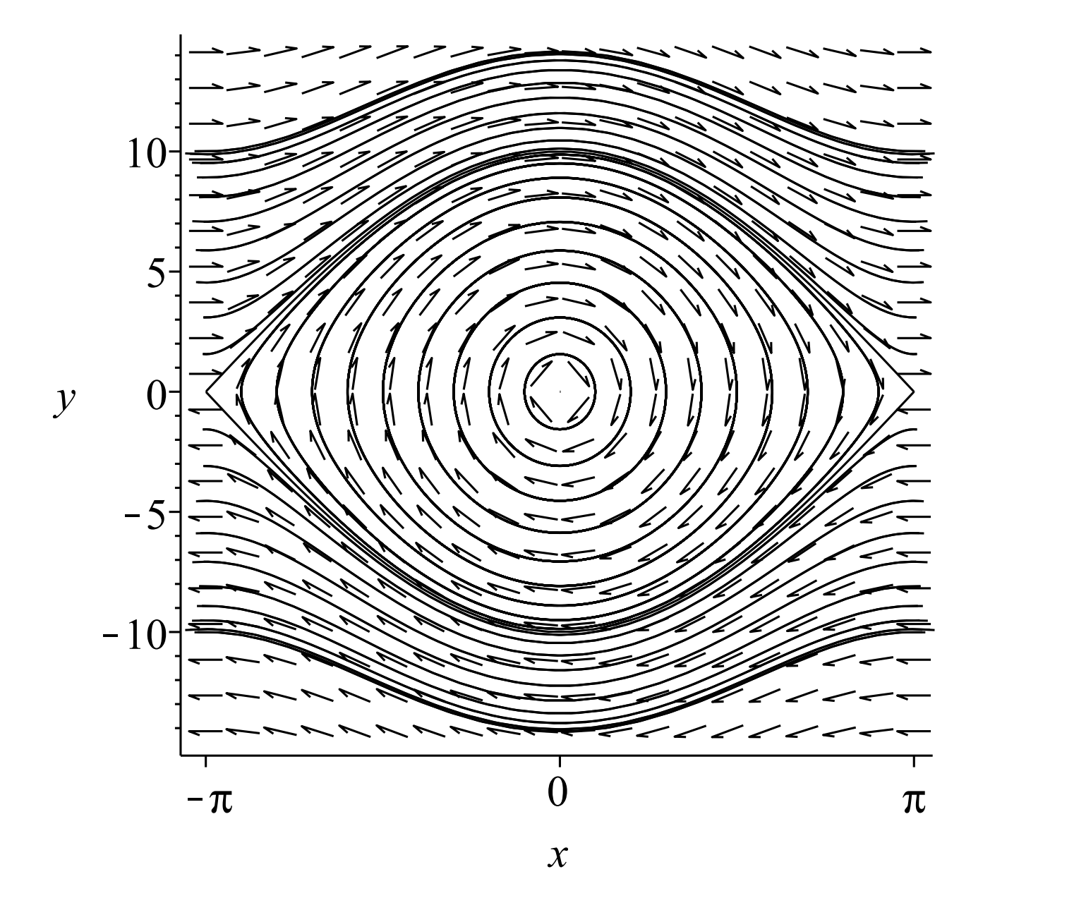
In Figure \(\PageIndex{7}\) we show the phase plane for the undamped nonlinear pendulum with \(\omega=1.25\). We see that we have a mixture of centers and saddles. There are orbits for which there is periodic motion. In the case that \(\theta = \pi\) we have an inverted pendulum. This is an unstable position and this is reflected in the presence of saddle points, especially if the pendulum is constructed using a massless rod.

Figure \(\PageIndex{7}\): Phase plane for the undamped nonlinear pendulum. Solution curves are shown for initial conditions \(\left(x_{0}, y_{0}\right)=(0,3),(0,2),(0,1),(5,1)\).

There are also unbounded orbits, going through all possible angles. These correspond to the mass spinning around the pivot in one direction forever due to initially having large enough energies.

We have indicated in the figure solution curves with the initial conditions \(\left(x_{0}, y_{0}\right)=(0,3),(0,2),(0,1),(5,1)\). These show the various types of motions that we have described.

Figure \(\PageIndex{8}\): Phase plane for the damped nonlinear pendulum. Solution curves are shown for initial conditions \(\left(x_{0}, y_{0}\right)=(0,3),(0,2),(0,1),(5,1) \).

When there is damping, we see that we can have a variety of other behaviors as seen in Figure \(\PageIndex{8}\). In this example we have set \(b=0.08\) and \(\omega=1.25 \). We see that energy loss results in the mass settling around one of the stable fixed points. This leads to an understanding as to why there are an infinite number of equilibria, even though physically the mass traces out a bound set of Cartesian points. We have indicated in the Figure \(\PageIndex{8}\) solution curves with the initial conditions \(\left(x_{0}, y_{0}\right)=(0,3),(0,2),(0,1),(5,1)\).

In Figure \(\PageIndex{9}\) we show a region of the phase plane which corresponds to oscillations about \(x=0\). For small angles the pendulum oscillates following somewhat elliptical orbits. As the angles get larger, due to greater initial energies, these orbits begin to change from ellipses to other periodic orbits. There is a limiting orbit, beyond which one has unbounded motion. The limiting orbit connects the saddle points on either side of the center. The curve is called a separatrix and being that these trajectories connect two saddles, they are often referred to as heteroclinic orbits.

Figure \(\PageIndex{9}\): Several orbits in the phase plane for the undamped nonlinear pendulum with \(\omega=5.0\). The orbits surround a center at \((0,0)\). At the edges there are saddle points, \((\pm \pi, 0)\).

(Heteroclinc orbits and separatrices). In Figures \(\PageIndex{10}\) we show more orbits, including both bound and unbound motion beyond the interval \(x \in[-\pi, \pi]\). For both plots we have chosen \(\omega=5\) and the same set of initial conditions, \(x(0)=\pi k / 10, k=\) \(-20, \ldots, 20\). for \(y(0)=0, \pm 10\). The time interval is taken for \(t \in[-3,3]\). The only difference is that in the damped case we have \(b=0.5 \). In these plots one can see what happens to the heteroclinic orbits and nearby unbounded orbits under damping.

Figure \(\PageIndex{10}\): Several orbits in the phase plane for the undamped nonlinear pendulum with \(\omega=5.0\).

Before leaving this problem, we should note that the orbits in the phase plane for the undamped nonlinear pendulum can be obtained graphically. Recall from Equation 7.9.6, the total mechanical energy for the nonlinear pendulum is

\[E=\dfrac{1}{2} m L^{2} \dot{\theta}^{2}+m g L(1-\cos \theta) \nonumber \]

From this equation we obtained Equation 7.9.7,

\[\dfrac{1}{2} \dot{\theta}^{2}-\omega^{2} \cos \theta=-\omega^{2} \cos \theta_{0} \nonumber \]

Figure \(\PageIndex{11}\): Several orbits in the phase plane for the damped nonlinear pendulum with \(\omega=5.0\) and \(b=0.5\).

Letting \(y=\dot{\theta}, x=\theta\), and defining \(z=-\omega^{2} \cos \theta_{0}\), this equation can be Written as

\[\dfrac{1}{2} y^{2}-\omega^{2} \cos x=z \nonumber \]

For each energy \((z)\), this gives a constant energy curve. Plotting the family of energy curves we obtain the phase portrait shown in Figure \(\PageIndex{12}\).

Figure \(\PageIndex{12}\): A family of energy curves in the phase plane for \(\dfrac{1}{2} \dot{\theta}^{2}-\omega^{2} \cos \theta=z\). Here we took \(\omega=1.0\) and \(z \in[-5,15]\).