2.1: Linear Equations

Last updated
Save as PDF

Page ID: 2133

$ \newcommand{\vecs}[1]{\overset { \scriptstyle \rightharpoonup} {\mathbf{#1}} } $ $ \newcommand{\vecd}[1]{\overset{-\!-\!\rightharpoonup}{\vphantom{a}\smash {#1}}} $$\newcommand{\id}{\mathrm{id}}$ $ \newcommand{\Span}{\mathrm{span}}$ $ \newcommand{\kernel}{\mathrm{null}\,}$ $ \newcommand{\range}{\mathrm{range}\,}$ $ \newcommand{\RealPart}{\mathrm{Re}}$ $ \newcommand{\ImaginaryPart}{\mathrm{Im}}$ $ \newcommand{\Argument}{\mathrm{Arg}}$ $ \newcommand{\norm}[1]{\| #1 \|}$ $ \newcommand{\inner}[2]{\langle #1, #2 \rangle}$ $ \newcommand{\Span}{\mathrm{span}}$ $\newcommand{\id}{\mathrm{id}}$ $ \newcommand{\Span}{\mathrm{span}}$ $ \newcommand{\kernel}{\mathrm{null}\,}$ $ \newcommand{\range}{\mathrm{range}\,}$ $ \newcommand{\RealPart}{\mathrm{Re}}$ $ \newcommand{\ImaginaryPart}{\mathrm{Im}}$ $ \newcommand{\Argument}{\mathrm{Arg}}$ $ \newcommand{\norm}[1]{\| #1 \|}$ $ \newcommand{\inner}[2]{\langle #1, #2 \rangle}$ $ \newcommand{\Span}{\mathrm{span}}$

Let us begin with the linear homogeneous equation
\begin{equation}
\label{homtwo}
a_1(x,y)u_x+a_2(x,y)u_y=0.
\end{equation}
Assume there is a $C^1$-solution $z=u(x,y)$. This function defines a surface $S$ which has at $P=(x,y,u(x,y))$ the normal
$$
{\bf N}=\frac{1}{\sqrt{1+|\nabla u|^2}}(-u_x,-u_y,1)
$$
and the tangential plane defined by
$$
\zeta-z=u_x(x,y)(\xi-x)+u_y(x,y)(\eta-y).
$$
Set $p=u_x(x,y)$, $q=u_y(x,y)$ and $z=u(x,y)$. The tuple $(x,y,z,p,q)$ is called surface element and the tuple $(x,y,z)$ support of the surface element. The tangential plane is defined by the surface element. On the other hand, differential equation (\ref{homtwo})
$$
a_1(x,y)p+a_2(x,y)q=0
$$
defines at each support $(x,y,z)$ a bundle of planes if we consider all $(p,q)$ satisfying this equation. For fixed $(x,y)$, this family of planes $\Pi(\lambda)=\Pi(\lambda;x,y)$ is defined by a one parameter family of ascents $p(\lambda)=p(\lambda;x,y)$, $q(\lambda)=q(\lambda;x,y)$.
The envelope of these planes is a line since
$$
a_1(x,y)p(\lambda)+a_2(x,y)q(\lambda)=0,
$$
which implies that the normal ${\bf N}(\lambda)$ on $\Pi(\lambda)$ is perpendicular on $(a_1,a_2,0)$.

Consider a curve ${\bf x}(\tau)=(x(\tau),y(\tau),z(\tau))$ on $\mathcal S$, let
$T_{{\bf x}_0}$ be the tangential plane at ${\bf x}_0=(x(\tau_0),y(\tau_0),z(\tau_0))$ of $\mathcal S$
and consider on $T_{{\bf x}_0}$ the line
$$
L:\ \ l(\sigma)={\bf x}_0+\sigma{\bf x}'(\tau_0),\ \ \sigma\in\mathbb{R}^1,
$$
see Figure 2.1.1.

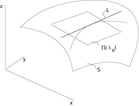
Figure 2.1.1: Curve on a surface

We assume $L$ coincides with the envelope, which is a line here, of the family of planes $\Pi(\lambda)$ at $(x,y,z)$. Assume that $T_{{\bf x}_0}=\Pi(\lambda_0)$ and consider two planes
\begin{eqnarray*}
\Pi(\lambda_0):\ \ \ z-z_0&=&(x-x_0)p(\lambda_0)+(y-y_0)q(\lambda_0)\\
\Pi(\lambda_0+h):\ \ \ z-z_0&=&(x-x_0)p(\lambda_0+h)+(y-y_0)q(\lambda_0+h).
\end{eqnarray*}
At the intersection $l(\sigma)$ we have
$$
(x-x_0)p(\lambda_0)+(y-y_0)q(\lambda_0)=(x-x_0)p(\lambda_0+h)+(y-y_0)q(\lambda_0+h).
$$
Thus,
$$
x'(\tau_0)p'(\lambda_0)+y'(\tau_0)q'(\lambda_0)=0.
$$
From the differential equation
$$
a_1(x(\tau_0),y(\tau_0))p(\lambda)+a_2(x(\tau_0),y(\tau_0))q(\lambda)=0
$$
it follows
$$
a_1p'(\lambda_0)+a_2q'(\lambda_0)=0.
$$
Consequently
$$
(x'(\tau),y'(\tau))=\frac{x'(\tau)}{a_1(x(\tau,y(\tau))}(a_1(x(\tau),y(\tau)),a_2(x(\tau),y(\tau)),
$$
since $\tau_0$ was an arbitrary parameter. Here we assume that $x'(\tau)\not=0$ and $a_1(x(\tau),y(\tau))\not=0$.

Then we introduce a new parameter $t$ by the inverse of $\tau=\tau(t)$, where
$$
t(\tau)=\int_{\tau_0}^\tau \frac{x'(s)}{a_1(x(s),y(s))}\ ds.
$$
It follows $x'(t)=a_1(x,y),\ y'(t)=a_2(x,y)$. We denote ${\bf x}(\tau(t))$ by ${\bf x}(t)$ again.

Now we consider the initial value problem
\begin{equation}
\label{chartwo}
x'(t)=a_1(x,y),\ \ y'(t)=a_2(x,y),\ \ x(0)=x_0,\ y(0)=y_0.
\end{equation}
From the theory of ordinary differential equations it follows (Theorem of Picard-Lindelöf) that there is a unique solution in a neighbourhood of $t=0$ provided the functions $a_1,\ a_2$ are in $C^1$. From this definition of the curves $(x(t),y(t))$ is follows that
the field of directions $(a_1(x_0,y_0),a_2(x_0,y_0))$ defines the slope of these curves at $(x(0),y(0))$.

Definition. The differential equations in (\ref{chartwo}) are called characteristic equations or characteristic system and solutions of the associated initial value problem are called characteristic curves.

Definition. A function $\phi(x,y)$ is said to be an integral of the characteristic system if $\phi(x(t),y(t))=const.$ for each characteristic curve. The constant depends on the characteristic curve considered.

Proposition 2.1. Assume $\phi\in C^1$ is an integral, then $u=\phi(x,y)$ is a solution of (\ref{homtwo}).

Proof. Consider for given $(x_0,y_0)$ the above initial value problem (\ref{chartwo}). Since $\phi(x(t),y(t))=const.$ it follows
$$
\phi_xx'+\phi_yy'=0
$$
for $ |t|<t_0$, $t_0>0$ and sufficiently small.
Thus
$$
\phi_x(x_0,y_0)a_1(x_0,y_0)+\phi_y(x_0,y_0)a_2(x_0,y_0)=0.
$$

$\Box$

Remark. If $\phi(x,y)$ is a solution of equation (\ref{homtwo}) then also $H(\phi(x,y))$, where $H(s)$ is a given $C^1$-function.

Examples

Example 2.1.1:

Consider
$$
a_1u_x+a_2u_y=0,
$$
where $a_1,\ a_2$ are constants. The system of characteristic equations is
$$
x'=a_1,\ y'=a_2.
$$
Thus the characteristic curves are parallel straight lines defined by
$$
x=a_1t+A,\ y=a_2t+B,
$$
where $A,\ B$ are arbitrary constants. From these equations it follows that
$$
\phi(x,y):=a_2x-a_1y
$$
is constant along each characteristic curve. Consequently, see Proposition 2.1, $u=a_2x-a_1y$ is a solution of the differential equation. From an exercise it follows that
\begin{equation}
\label{cyl}
u=H(a_2x-a_1y),
\end{equation}
where $H(s)$ is an arbitrary $C^1$-function, is also a solution. Since $u$ is constant when $a_2x-a_1y$ is constant, equation (\ref{cyl}) defines cylinder surfaces which are generated by parallel straight lines which are parallel to the $(x,y)$-plane, see Figure 2.1.2.

$Cylinder surfaces$
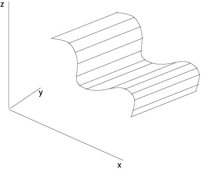
Figure 2.1.2: Cylinder surfaces

Example 2.1.2:

Consider the differential equation
$$
xu_x+yu_y=0.
$$
The characteristic equations are
$$
x'=x,\ y'=y,
$$
and the characteristic curves are given by
$$
x=Ae^t,\ y=Be^t,
$$
where $A,\ B$ are arbitrary constants. Then an integral is $y/x$, $x\not=0$, and for a given $C^1$-function the function $u=H(x/y)$ is a solution of the differential equation. If $y/x=const.$, then $u$ is constant. Suppose that $H'(s)>0$, for example, then $u$ defines right helicoids (in German: Wendelflächen), see Figure 2.1.3.

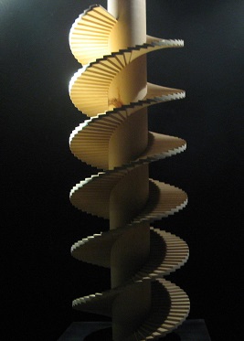
Figure 2.1.3: Right helicoid, $a^2<x^2+y^2<R^2$ (Museo Ideale Leonardo da Vinci, Italy)

Example 2.1.3:

Consider the differential equation
$$
yu_x-xu_y=0.
$$
The associated characteristic system is
$$
x'=y,\ y'=-x.
$$
If follows
$$
x'x+yy'=0,
$$
or, equivalently,
$$
\frac{d}{dt}(x^2+y^2)=0,
$$
which implies that $x^2+y^2=const.$ along each characteristic. Thus, rotationally symmetric surfaces defined by $u=H(x^2+y^2)$, where $H'\not=0$, are solutions of the differential equation.

Example 2.1.4:

The associated characteristic equations to
$$
ayu_x+bxu_y=0,
$$
where $a,\ b$ are positive constants,
are given by
$$
x'=ay,\ y'=bx.
$$
It follows $bxx'-ayy'=0$, or equivalently,
$$
\frac{d}{dt}(bx^2-ay^2)=0.
$$
Solutions of the differential equation are $u=H(bx^2-ay^2)$, which define surfaces which have a hyperbola as the intersection with planes parallel to the $(x,y)$-plane. Here $H(s)$ is an arbitrary $C^1$-function, $H'(s)\not=0$.

Contributors

Prof. Dr. Erich Miersemann (Universität Leipzig)
Integrated by Justin Marshall.