2.3: Nonlinear Equations in Two Variables

Here we consider equation

\begin{equation}
\label{nonlinear1}
F(x,y,z,p,q)=0,
\end{equation}

where \(z=u(x,y)\), \(p=u_x(x,y)\), \(q=u_y(x,y)\) and \(F\in C^2\) is given such that \(F_p^2+F_q^2\not=0\).

In contrast to the quasilinear case, this general nonlinear equation is more complicated.

Together with (\ref{nonlinear1}) we will consider the following system of ordinary equations which follow from considerations below as necessary conditions, in particular from the assumption that there is a solution of (\ref{nonlinear1}).

\begin{eqnarray}
\label{char1}
x'(t)&=&F_p\\
\label{char2}
y'(t)&=&F_q\\
\label{char3}
z'(t)&=&pF_p+qF_q\\
\label{char4}
p'(t)&=&-F_x-F_up\\
\label{char5}
q'(t)&=&-F_y-F_uq.
\end{eqnarray}

Definition. Equations (\ref{char1})--(\ref{char5}) are said to be characteristic equations of equation (\ref{nonlinear1}) and a solution

$$(x(t),y(t),z(t),p(t),q(t))\]

of the characteristic equations is called characteristic strip or Monge curve.

Figure 2.3.1: Gaspard Monge (Panthèon, Paris)

We will see, as in the quasilinear case, that the strips defined by the characteristic equations build the solution surface of the Cauchy initial value problem.

Let \(z=u(x,y)\) be a solution of the general nonlinear differential equation (\ref{nonlinear1}).

Let \((x_0,y_0,z_0)\) be fixed, then equation (\ref{nonlinear1}) defines a set of planes given by
\((x_0,y_0,z_0,p,q)\), i. e., planes given by \(z=v(x,y)\) which contain the point \((x_0,y_0,z_0)\)
and for which \(v_x=p\), \(v_y=q\) at \((x_0,y_0)\). In the case of quasilinear equations these set of planes is a bundle of planes which all contain a fixed straight line, see Section 2.1. In the general case of this section the situation is more complicated.

Consider the example

\begin{equation}
\label{monge1}
p^2+q^2=f(x,y,z),
\end{equation}

where \(f\) is a given positive function. Let \(E\) be a plane defined by \(z=v(x,y)\) and which contains \((x_0,y_0,z_0)\). Then the normal on the plane \(E\) directed downward is

$${\bf N}=\frac{1}{\sqrt{1+|\nabla v|^2}}(p,q,-1),\]

where \(p=v_x(x_0,y_0)\), \(q=v_y(x_0,y_0)\). It follows from (\ref{monge1}) that the normal \({\bf N}\) makes a constant angle with the \(z\)-axis, and the \(z\)-coordinate of \({\bf N}\) is constant, see Figure 2.3,2.

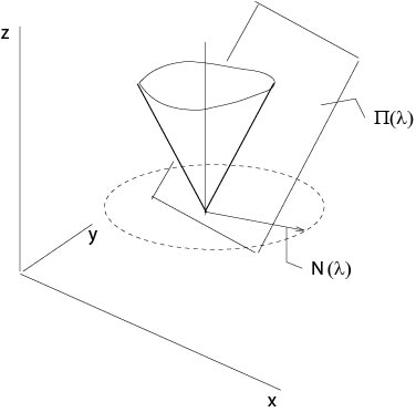
Figure 2.3.2: Monge cone in an example

Thus the endpoints of the normals fixed at \((x_0,y_0,z_0)\) define a circle parallel to the \((x,y)\)-plane, i. e., there is a cone which is the envelope of all these planes.

We assume that the general equation (\ref{nonlinear1}) defines such a Monge cone at each point in \(\mathbb{R}^3\). Then we seek a surface \(S\) which touches at each point its Monge cone, see Figure 2.3.3.

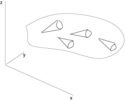
Figure 2.3.3: Monge cones

More precisely, we assume there exists, as in the above example, a one parameter \(C^1\)-family

$$p(\lambda)=p(\lambda;x,y,z),\ q(\lambda)=q(\lambda;x,y,z)\]

of solutions of (\ref{nonlinear1}). These \((p(\lambda),q(\lambda))\) define a family \(\Pi(\lambda)\) of planes.

Let

$${\bf x}(\tau)=(x(\tau),y(\tau),z(\tau))\]

be a curve on the surface \(S\) which touches at each point its Monge cone, see Figure 2.3.4. Thus we assume that at each point of the surface \(\mathcal S\) the associated tangent plane coincides with a plane from the family \(\Pi(\lambda)\) at this point.

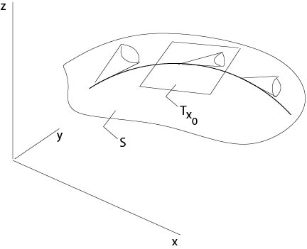
Figure 2.3.4: Monge cones along a curve on the surface

Consider the tangential plane \(T_{{\bf x}_0}\) of the surface \(S\) at \({\bf x}_0=(x(\tau_0),y(\tau_0),z(\tau_0))\). The straight line

$${\bf l}(\sigma)={\bf x}_0+\sigma {\bf x}'(\tau_0),\qquad -\infty<\sigma<\infty,\]

is an apothem (in German: Mantellinie) of the cone by assumption and is contained in the tangential plane \(T_{{\bf x}_0}\) as the tangent of a curve on the surface \(S\). It is defined through

\begin{equation}
\label{xl}
{\bf x}'(\tau_0)={\bf l}'(\sigma).
\end{equation}

The straight line \({\bf l}(\sigma)\) satisfies

$$l_3(\sigma)-z_0=(l_1(\sigma)-x_0)p(\lambda_0)+(l_2(\sigma)-y_0)q(\lambda_0),\]

since it is contained in the tangential plane \(T_{{\bf x}_0}\) defined by the slope \((p,q)\). It follows

$$l_3'(\sigma)=p(\lambda_0)l_1'(\sigma)+q(\lambda_0)l_2'(\sigma).\]

Together with (\ref{xl}) we obtain

\begin{equation}
\label{zpq}
z'(\tau)=p(\lambda_0)x'(\tau)+q(\lambda_0)y'(\tau).
\end{equation}

The above straight line \({\bf l}\) is the limit of the intersection line of two neighboring planes which envelopes the Monge cone:

\begin{eqnarray*}
z-z_0&=&(x-x_0)p(\lambda_0)+(y-y_0)q(\lambda_0)\\
z-z_0&=&(x-x_0)p(\lambda_0+h)+(y-y_0)q(\lambda_0+h).
\end{eqnarray*}

On the intersection one has

$$(x-x_0)p(\lambda)+(y-y_0)q(\lambda_0)=(x-x_0)p(\lambda_0+h)+(y-y_0)q(\lambda_0+h).\]

Let \(h\to 0\), it follows

$$(x-x_0)p'(\lambda_0)+(y-y_0)q'(\lambda_0)=0.\]

Since \(x=l_1(\sigma)\), \(y=l_2(\sigma)\) in this limit position, we have

$$p'(\lambda_0)l_1'(\sigma)+q'(\lambda_0)l_2'(\sigma)=0,\]

and it follows from (\ref{xl}) that

\begin{equation}
\label{pxqy}
p'(\lambda_0)x'(\tau)+q'(\lambda_0)y'(\tau)=0.
\end{equation}

From the differential equation \(F(x_0,y_0,z_0,p(\lambda),q(\lambda))=0\) we see that
\begin{equation}
\label{Fpq}
F_pp'(\lambda)+F_qq'(\lambda)=0.
\end{equation}

Assume \(x'(\tau_0)\not=0\) and \(F_p\not=0\), then we obtain from (\ref{pxqy}), (\ref{Fpq})
\begin{equation*}
%\label{q1}
\frac{y'(\tau_0)}{x'(\tau_0)}=\frac{F_q}{F_p},
\end{equation*}
and from (\ref{zpq}) (\ref{Fpq}) that
\begin{equation*}
%\label{q2}
\frac{z'(\tau_0)}{x'(\tau_0)}=p+q\frac{F_q}{F_p}.
\end{equation*}
It follows, since \(\tau_0\) was an arbitrary fixed parameter,
\begin{eqnarray*}
{\bf x}'(\tau)&=&(x'(\tau),y'(\tau),z'(\tau))\\
&=&\left(x'(\tau),x'(\tau)\frac{F_q}{F_p},x'(\tau)\left(p+q\frac{F_q}{F_p}\right)\right)\\
&=&\frac{x'(\tau)}{F_p}(F_p,F_q,pF_p+qF_q),
\end{eqnarray*}
i. e., the tangential vector \({\bf x}'(\tau)\) is proportional to \((F_p,F_q,pF_p+qF_q)\).
Set
$$
a(\tau)=\frac{x'(\tau)}{F_p},
$$
where \(F=F(x(\tau),y(\tau),z(\tau),p(\lambda(\tau)),q(\lambda(\tau)))\). Introducing the new parameter \(t\) by the inverse of \(\tau=\tau(t)\), where
$$
t(\tau)=\int_{\tau_0}^\tau\ a(s)\ ds,
$$
we obtain the characteristic equations (\ref{char1})--(\ref{char3}).
Here we denote \({\bf x}(\tau(t))\) by \({\bf x}(t)\) again.
From the differential equation (\ref{nonlinear1}) and from (\ref{char1})--(\ref{char3}) we get equations (\ref{char4}) and (\ref{char5}). Assume the surface \(z=u(x,y)\) under consideration is in \(C^2\), then
\begin{eqnarray*}
F_x+F_zp+F_pp_x+F_qp_y&=&0,\ \ (q_x=p_y)\\
F_x+F_zp+x'(t)p_x+y'(t)p_y&=&0\\
F_x+F_zp+p'(t)&=&0
\end{eqnarray*}
since \(p=p(x,y)=p(x(t),y(t))\) on the curve \({\bf x}(t)\). Thus equation (\ref{char4}) of the characteristic system is shown. Differentiating the differential equation (\ref{nonlinear1}) with respect to \(y\), we get finally equation (\ref{char5}).

Remark. In the previous quasilinear case
$$
F(x,y,z,p,q)=a_1(x,y,z)p+a_2(x,y,z)q-a_3(x,y,z)
$$
the first three characteristic equations are the same:
$$
x'(t)=a_1(x,y,z),\ y'(t)=a_2(x,y,z),\ z'(t)=a_3(x,y,z).
$$
The point is that the right hand sides are independent on \(p\) or \(q\). It follows from Theorem 2.1 that there exists a solution of the Cauchy initial value problem provided the initial data are non-characteristic. That is, we do not need the other remaining two characteristic equations.

The other two equations (\ref{char4}) and (\ref{char5}) are satisfied in this quasilinear case automatically if there is a solution of the equation, see the above derivation of these equations.

The geometric meaning of the first three characteristic differential equations (\ref{char1})--(\ref{char5}) is the following one. Each point of the curve
$$
{\mathcal A}:\quad (x(t),y(t),z(t))
$$
corresponds a tangential plane with the normal direction \((-p,-q,1)\) such that
$$
z'(t)=p(t)x'(t)+q(t)y'(t).
$$
This equation is called strip condition. On the other hand, let \(z=u(x,y)\) defines a surface, then \(z(t):=u(x(t),y(t))\) satisfies the strip condition, where \(p=u_x\) and \(q=u_y\), that is, the ''scales'' defined by the normals fit together.

Proposition 2.3. \(F(x,y,z,p,q)\) is an integral, i. e., it is constant along each characteristic curve.

Proof.
\begin{eqnarray*}
\frac{d}{dt}F(x(t),y(t),z(t),p(t),q(t))&=&F_xx'+F_yy'+F_zz'+F_pp'+F_qq'\\
&=&F_xF_p+F_yF_q+pF_zF_p+qF_zF_q\\
&&-F_pf_x-F_pF_zp-F_qF_y-F_qF_zq\\
&=&0.
\end{eqnarray*}

\(\Box\)

Corollary. Assume \(F(x_0,y_0,z_0,p_0,q_0)=0\), then \(F=0\) along characteristic curves with the initial data \((x_0,y_0,z_0,p_0,q_0)\).

Proposition 2.4.
Let \(z=u(x,y)\), \(u\in C^2\), be a solution of the nonlinear equation (\ref{nonlinear1}). Set
$$
z_0=u(x_0,y_0,)\ p_0=u_x(x_0,y_0),\ q_0=u_y(x_0,y_0).
$$
Then the associated characteristic strip is in the surface \(\mathcal{S}\), defined by \(z=u(x,y)\).
Thus
\begin{eqnarray*}
z(t)&=&u(x(t),y(t))\\
p(t)&=&u_x(x(t),y(t))\\
q(t)&=&u_y(x(t),y(t)),
\end{eqnarray*}
where \((x(t),y(t),z(t),p(t),q(t))\) is the solution of the characteristic system (\ref{char1})--(\ref{char5}) with initial data \((x_0,y_0,z_0,p_0,q_0)\)

Proof. Consider the initial value problem
\begin{eqnarray*}
x'(t)&=&F_p(x,y,u(x,y),u_x(x,y),u_y(x,y))\\
y'(t)&=&F_q(x,y,u(x,y),u_x(x,y),u_y(x,y))
\end{eqnarray*}
with the initial data \(x(0)=x_0\), \(y(0)=y_0\). We will show that
$$
(x(t),y(t),u(x(t),y(t)),u_x(x(t),y(t)),u_y(x(t),y(t)))
$$
is a solution of the characteristic system. We recall that the solution exists and is uniquely determined.

Set \(z(t)=u(x(t),y(t))\), then \((x(t),y(t),z(t))\subset\mathcal{S}\), and
$$
z'(t)=u_xx'(t)+u_yy'(t)=u_xF_p+u_yF_q.
$$
Set \(p(t)=u_x(x(t),y(t)),\ q(t)=u_y(x(t),y(t))\), then
\begin{eqnarray*}
p'(t)&=&u_{xx}F_p+u_{xy}F_q\\
q'(t)&=&u_{yx}F_p+u_{yy}F_q.
\end{eqnarray*}
Finally, from the differential equation \(F(x,y,u(x,y),u_x(x,y),u_y(x,y))=0\) it follows
\begin{eqnarray*}
p'(t)&=&-F_x-F_up\\
q'(t)&=&-F_y-F_uq.
\end{eqnarray*}

\(\Box\)

Contributors and Attributions

• Prof. Dr. Erich Miersemann (Universität Leipzig)

• Integrated by Justin Marshall.