2.2.2: Initial Value Problem of Cauchy

Consider again the quasilinear equation

($\star$) $a_1(x,y,u)u_x+a_2(x,y,u)u_y=a_3(x,y,u)$.

Let
$$\Gamma:\ \ x=x_0(s),\ y=y_0(s),\ z=z_0(s), \ s_1\le s\le s_2,\ -\infty<s_1<s_2<+\infty$$
be a regular curve in $\mathbb{R}^3$ and denote by $\mathcal{C}$ the orthogonal projection of $\Gamma$ onto the $(x,y)$-plane, i. e.,
$$
\mathcal{C}:\ \ x=x_0(s),\ \ y=y_0(s).
\]

Initial value problem of Cauchy: Find a $C^1$-solution $u=u(x,y)$ of $(\star)$ such that $u(x_0(s),y_0(s))=z_0(s)$, i. e., we seek a surface $\mathcal{S}$ defined by $z=u(x,y)$ which contains the curve $\Gamma$.

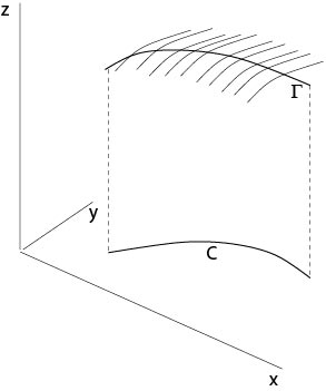
Figure 2.2.2.1: Cauchy initial value problem

Definition. The curve $\Gamma$ is said to be non-characteristic if
$$
x_0'(s)a_2(x_0(s),y_0(s))-y_0'(s)a_1(x_0(s),y_0(s))\not=0.
\]

Theorem 2.1. Assume $a_1,\ a_2,\ a_2\in C^1$ in their arguments, the initial data $x_0,\ y_0,\ z_0\in C^1[s_1,s_2]$ and $\Gamma$ is non-characteristic.

Then there is a neighborhood of $\cal{C}$ such that there exists exactly one solution $u$ of the Cauchy initial value problem.

Proof. (i) Existence. Consider the following initial value problem for the system of characteristic equations to ($\star$):
$$\begin{eqnarray*} x'(t)&=&a_1(x,y,z)\\ y'(t)&=&a_2(x,y,z)\\ z'(t)&=&a_3(x,y,z) \end{eqnarray*}$$
with the initial conditions
$$\begin{eqnarray*} x(s,0)&=&x_0(s)\\ y(s,0)&=&y_0(s)\\ z(s,0)&=&z_0(s). \end{eqnarray*}$$
Let $x=x(s,t)$, $y=y(s,t)$, $z=z(s,t)$ be the solution, $s_1\le s\le s_2$, $|t|<\eta$ for an $\eta>0$. We will show that this set of curves, see Figure 2.2.2.1, defines a surface. To show this, we consider the inverse functions $s=s(x,y)$, $t=t(x,y)$ of $x=x(s,t)$, $y=y(s,t)$ and show that $z(s(x,y),t(x,y))$ is a solution of the initial problem of Cauchy. The inverse functions $s$ and $t$ exist in a neighborhood of $t=0$ since
$$\det \frac{\partial(x,y)}{\partial(s,t)}\Big|_{t=0}= \left|\begin{array}{cc}x_s&x_t\\y_s&y_t\end{array}\right|_{t=0} =x_0'(s)a_2-y_0'(s)a_1\not=0,$$
and the initial curve $\Gamma$ is non-characteristic by assumption.

Set
$$u(x,y):=z(s(x,y),t(x,y)),$$
then $u$ satisfies the initial condition since
$$u(x,y)|_{t=0}=z(s,0)=z_0(s).$$
The following calculation shows that $u$ is also a solution of the differential equation ($\star$).
$$\begin{eqnarray*} a_1u_x+a_2u_y&=&a_1(z_ss_x+z_tt_x)+a_2(z_ss_y+z_tt_y)\\ &=&z_s(a_1s_x+a_2s_y)+z_t(a_1t_x+a_2t_y)\\ &=&z_s(s_xx_t+s_yy_t)+z_t(t_xx_t+t_yy_t)\\ &=&a_3 \end{eqnarray*}$$
since $0=s_t=s_xx_t+s_yy_t$ and $1=t_t=t_xx_t+t_yy_t$.

(ii) Uniqueness. Suppose that $v(x,y)$ is a second solution. Consider a point $(x',y')$ in a neighborhood of the curve $(x_0(s),y(s))$, $s_1-\epsilon\le s\le s_2+\epsilon$, $\epsilon>0$ small. The inverse parameters are $s'=s(x',y')$, $t'=t(x',y')$, see Figure 2.2.2.2.

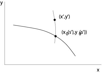
Figure 2.2.2.2: Uniqueness proof

Let
$${\mathcal{A}}:\ \ x(t):=x(s',t),\ y(t):=y(s',t),\ z(t):=z(s',t)$$
be the solution of the above initial value problem for the characteristic differential equations with the initial data
$$x(s',0)=x_0(s'),\ y(s',0)=y_0(s'),\ z(s',0)=z_0(s').$$
According to its construction this curve is on the surface $\mathcal{S}$ defined by $u=u(x,y)$ and $u(x',y')=z(s',t')$. Set
$$\psi(t):=v(x(t),y(t))-z(t),$$
then
$$\begin{eqnarray*} \psi'(t)&=&v_xx'+v_yy'-z'\\ &=&x_xa_1+v_ya_2-a_3=0 \end{eqnarray*}$$
and
$$\psi(0)=v(x(s',0),y(s',0))-z(s',0) =0$$
since $v$ is a solution of the differential equation and satisfies the initial condition by assumption. Thus, $\psi(t)\equiv0$, i. e.,
$$v(x(s',t),y(s',t))-z(s',t)=0.$$
Set $t=t'$, then
$$v(x',y')-z(s',t')=0,$$
which shows that $v(x',y')=u(x',y')$ because of $z(s',t')=u(x',y')$.

$\Box$

Remark. In general, there is no uniqueness if the initial curve $\Gamma$ is a characteristic curve, see an exercise and Figure 2.2.2.3, which illustrates this case.

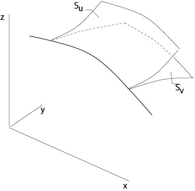
Figure 2.2.2.3: Multiple solutions

Examples

Example 2.2.2.1:

Consider the Cauchy initial value problem
$$u_x+u_y=0$$
with the initial data
$$x_0(s)=s,\ y_0(s)=1,\ z_0(s)\ \mbox{is a given}\ C^1\mbox{-function}.$$
These initial data are non-characteristic since $y_0'a_1-x_0'a_2=-1$. The solution of the associated system of characteristic equations
$$x'(t)=1,\ y'(t)=1,\ u'(t)=0$$
with the initial conditions
$$x(s,0)=x_0(s),\ y(s,0)=y_0(s),\ z(s,0)=z_0(s)$$
is given by
$$x=t+x_0(s),\ y=t+y_0(s),\ z=z_0(s) ,$$
i. e.,
$$x=t+s,\ y=t+1,\ z=z_0(s).$$
It follows $s=x-y+1,\ t=y-1$ and that $u=z_0(x-y+1)$ is the solution of the Cauchy initial value problem.

Example 2.2.2.2:

A problem from kinetics in chemistry. Consider for $x\ge0$, $y\ge0$ the problem
$$u_x+u_y=\left(k_0e^{-k_1x}+k_2\right)(1-u)$$
with initial data
$$u(x,0)=0,\ x>0,\ \mbox{and}\ u(0,y)=u_0(y),\ y>0.$$
Here the constants $k_j$ are positive, these constants define the velocity of the reactions in consideration, and the function $u_0(y)$ is given. The variable $x$ is the time and $y$ is the height of a tube, for example, in which the chemical reaction takes place, and $u$ is the concentration of the chemical substance.

In contrast to our previous assumptions, the initial data are not in $C^1$. The projection ${\mathcal C}_1\cup {\mathcal C}_2$ of the initial curve onto the $(x,y)$-plane has a corner at the origin, see Figure 2.2.2.4.

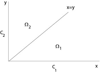
Figure 2.2.2.4: Domains to the chemical kinetics example

The associated system of characteristic equations is
$$x'(t)=1,\ y'(t)=1,\ z'(t)=\left(k_0e^{-k_1x}+k_2\right)(1-z).$$
It follows $x=t+c_1$, $y=t+c_2$ with constants $c_j$. Thus the projection of the characteristic curves on the $(x,y)$-plane are straight lines parallel to $y=x$. We will solve the initial value problems in the domains $\Omega_1$ and $\Omega_2$, see Figure 2.2.2.4, separately.

(i) The initial value problem in $\Omega_1$. The initial data are
$$x_0(s)=s,\ y_0(s)=0, \ z_0(0)=0,\ s\ge 0.$$
It follows
$$x=x(s,t)=t+s,\ y=y(s,t)=t.$$
Thus
$$z'(t)=(k_0e^{-k_1(t+s)}+k_2)(1-z),\ z(0)=0.$$
The solution of this initial value problem is given by
$$z(s,t)=1-\exp\left(\frac{k_0}{k_1}e^{-k_1(s+t)}-k_2t-\frac{k_0}{k_1}e^{-k_1s}\right).$$
Consequently
$$u_1(x,y)=1-\exp\left(\frac{k_0}{k_1}e^{-k_1x}-k_2y-{k_0}{k_1}e^{-k_1(x-y)}\right)$$
is the solution of the Cauchy initial value problem in $\Omega_1$. If time $x$ tends to $\infty$, we get the limit
$$
\lim_{x\to\infty} u_1(x,y)=1-e^{-k_2y}.
\]

(ii) The initial value problem in $\Omega_2$. The initial data are here

$$x_0(s)=0,\ y_0(s)=s, \ z_0(0)=u_0(s),\ s\ge 0.$$
It follows
$$x=x(s,t)=t,\ y=y(s,t)=t+s.$$
Thus
$$z'(t)=(k_0e^{-k_1t}+k_2)(1-z),\ z(0)=0.$$
The solution of this initial value problem is given by
$$z(s,t)=1-(1-u_0(s))\exp\left(\frac{k_0}{k_1}e^{-k_1t}-k_2t-\frac{k_0}{k_1}\right).$$
Consequently
$$u_2(x,y)=1-(1-u_0(y-x))\exp\left(\frac{k_0}{k_1}e^{-k_1x}-k_2x-\frac{k_0}{k_1}\right)$$
is the solution in $\Omega_2$.

If $x=y$, then
$$\begin{eqnarray*} u_1(x,y)&=&1-\exp\left(\frac{k_0}{k_1}e^{-k_1x}-k_2x-\frac{k_0}{k_1}\right)\\ u_2(x,y)&=&1-(1-u_0(0))\exp\left(\frac{k_0}{k_1}e^{-k_1x}-k_2x-\frac{k_0}{k_1}\right). \end{eqnarray*}$$
If $u_0(0)>0$, then $u_1<u_2$ if $x=y$, i. e., there is a jump of the concentration of the substrate along its burning front defined by $x=y$.

Remark. Such a problem with discontinuous initial data is called Riemann problem. See an exercise for another Riemann problem.

The case that a solution of the equation is known

Here we will see that we get immediately a solution of the Cauchy initial value problem if a solution of the homogeneous linear equation
$$a_1(x,y)u_x+a_2(x,y)u_y=0$$
is known.

Let
$$x_0(s),\ y_0(s),\ z_0(s),\ s_1<s<s_2$$
be the initial data and let $u=\phi(x,y)$ be a solution of the differential equation. We assume that
$$\phi_x(x_0(s),y_0(s))x_0'(s)+\phi_y(x_0(s),y_0(s))y_0'(s)\not=0$$
is satisfied. Set
$$g(s)=\phi(x_0(s),y_0(s))$$
and let $s=h(g)$ be the inverse function.

The solution of the Cauchy initial problem is given by $u_0\left(h(\phi(x,y))\right)$.

This follows since in the problem considered a composition of a solution is a solution again, see an exercise, and since
$$
u_0\left(h(\phi(x_0(s),y_0(s))\right)=u_0(h(g))=u_0(s).
\]

Example 2.2.2.3:

Consider equation
$$u_x+u_y=0$$
with initial data
$$x_0(s)=s,\ y_0(s)=1,\ u_0(s)\ \mbox{is a given function}.$$
A solution of the differential equation is $\phi(x,y)=x-y$. Thus
$$\phi((x_0(s),y_0(s))=s-1$$
and
$$u_0(\phi+1)=u_0(x-y+1)$$
is the solution of the problem.

Contributors and Attributions

• Prof. Dr. Erich Miersemann (Universität Leipzig)

• Integrated by Justin Marshall.