
8.1: Fixed Points and Stability
- Page ID
- 90428

One Dimension
Consider the one-dimensional differential equation for \(x = x(t)\) given by \[\label{eq:1}\overset{.}{x}=f(x).\]
We say that \(x_*\) is a fixed point, or equilibrium point, of \(\eqref{eq:1}\) if \(f(x_*) = 0\). At the fixed point, \(\overset{.}{x} = 0\). The terminology fixed point is used since the solution to \(\eqref{eq:1}\) with initial condition \(x(0) = x_*\) is \(x(t) = x_*\) for all time \(t\).
A fixed point, however, can be stable or unstable. A fixed point is said to be stable if a small perturbation of the solution from the fixed point decays in time; it is said to be unstable if a small perturbation grows in time. We can determine stability by a linear analysis. Let \(x = x_* +\epsilon (t)\), where \(\epsilon\) represents a small perturbation of the solution from the fixed point \(x_*\). Because \(x_*\) is a constant, \(\overset{.}{x}=\overset{.}{\epsilon}\); and because \(x_*\) is a fixed point, \(f(x_*) = 0\). Taylor series expanding about \(\epsilon = 0\), we have \[\begin{aligned}\overset{.}{\epsilon}&=f(x_*+\epsilon) \\ &=f(x_*)+\epsilon f'(x_*)+\ldots \\ &=\epsilon f'(x_*)+\ldots\end{aligned}\]
The omitted terms in the Taylor series expansion are proportional to \(\epsilon^2\), and can be made negligible over a short time interval with respect to the kept term, proportional to \(\epsilon\), by taking \(\epsilon (0)\) sufficiently small. Therefore, at least over short times, the differential equation to be considered, \(\overset{.}{\epsilon}= f ' (x_*)\epsilon\), is linear and has by now the familiar solution \[\epsilon (t)=\epsilon (0)e^{f'(x_*)t}.\nonumber\]
The perturbation of the fixed point solution \(x(t) = x_*\) thus decays exponentially if \(f' (x_*) < 0\), and we say the fixed point is stable. If \(f' (x_*) > 0\), the perturbation grows exponentially and we say the fixed point is unstable. If \(f' (x_*) = 0\), we say the fixed point is marginally stable, and the next higher-order term in the Taylor series expansion must be considered.
Find all the fixed points of the logistic equation \(\overset{.}{x} = x(1 − x)\) and determine their stability.
Solution
There are two fixed points at which \(\overset{.}{x} = 0\), given by \(x_* = 0\) and \(x_* = 1\). Stability of these equilibrium points may be determined by considering the derivative of \(f(x) = x(1 − x)\). We have \(f' (x) = 1 − 2x\). Therefore, \(f' (0) = 1 > 0\) so that \(x_* = 0\) is an unstable fixed point, and \(f' (1) = −1 < 0\) so that \(x_* = 1\) is a stable fixed point. Indeed, we have previously found that all solutions approach the stable fixed point asymptotically.
Two Dimensions
The idea of fixed points and stability can be extended to higher-order systems of odes. Here, we consider a two-dimensional system and will need to make use of the two-dimensional Taylor series expansion of a function \(F(x, y)\) about the origin. In general, the Taylor series of \(F(x, y)\) is given by \[F(x,y)=F+x\frac{\partial F}{\partial x}+y\frac{\partial F}{\partial y}+\frac{1}{2}\left(x^2\frac{\partial ^2F}{\partial x^2}+2xy\frac{\partial ^2F}{\partial x\partial y}+y^2\frac{\partial^2F}{\partial y^2}\right)+\ldots,\nonumber\] where the function \(F\) and all of its partial derivatives on the right-hand-side are evaluated at the origin. Note that the Taylor series is constructed so that all partial derivatives of the left-hand-side match those of the right-hand-side at the origin.
We now consider the two-dimensional system given by \[\label{eq:2}\overset{.}{x}=f(x,y),\quad\overset{.}{y}=g(x,y).\]
The point \((x_*, y_*)\) is said to be a fixed point of \(\eqref{eq:2}\) if \(f(x_*, y_*) = 0\) and \(g(x_*, y_*) = 0\). Again, the local stability of a fixed point can be determined by a linear analysis. We let \(x(t) = x_* + \epsilon (t)\) and \(y(t) = y_* + \delta (t)\), where \(\epsilon\) and \(\delta\) are small independent perturbations from the fixed point. Making use of the two dimensional Taylor series of \(f(x, y)\) and \(g(x, y)\) about the fixed point, or equivalently about \((\epsilon , \delta ) = (0, 0)\), we have \[\begin{aligned}\overset{.}{\epsilon}&=f(x_*+\epsilon ,y_*+\delta ) \\ &=f+\epsilon\frac{\partial f}{\partial x}+\delta\frac{\partial f}{\partial y}+\ldots \\ &=\epsilon\frac{\partial f}{\partial x}+\delta\frac{\partial f}{\partial y}+\ldots \\ \delta &=g(x_*+\epsilon ,y_*+\delta ) \\ &=g+\epsilon\frac{\partial g}{\partial x}+\delta\frac{\partial g}{\partial y}+\ldots \\ &=\epsilon\frac{\partial g}{\partial x}+\delta\frac{\partial g}{\partial y}+\ldots,\end{aligned}\]
where in the Taylor series \(f,\: g\) and all their partial derivatives are evaluated at the fixed point \((x_*, y_*)\). Neglecting higher-order terms in the Taylor series, we thus have a system of odes for the perturbation, given in matrix form as \[\label{eq:3}\frac{d}{dt}\left(\begin{array}{c}\epsilon \\ \delta\end{array}\right)=\left(\begin{array}{cc}\frac{\partial f}{\partial x}&\frac{\partial f}{\partial y} \\ \frac{\partial g}{\partial x}&\frac{\partial g}{\partial y}\end{array}\right)\left(\begin{array}{c}\epsilon \\ \delta\end{array}\right).\]
The two-by-two matrix in \(\eqref{eq:3}\) is called the Jacobian matrix at the fixed point. An eigenvalue analysis of the Jacobian matrix will typically yield two eigenvalues \(\lambda_1\) and \(\lambda_2\). These eigenvalues may be real and distinct, complex conjugate pairs, or repeated. The fixed point is stable (all perturbations decay exponentially) if both eigenvalues have negative real parts. The fixed point is unstable (some perturbations grow exponentially) if at least one of the eigenvalues has a positive real part. Fixed points can be further classified as stable or unstable nodes, unstable saddle points, stable or unstable spiral points, or stable or unstable improper nodes.
Find all the fixed points of the nonlinear system \(\overset{.}{x}= x(3 − x − 2y)\), \(\overset{.}{y} = y(2 − x − y)\), and determine their stability.
Solution
The fixed points are determined by solving \[f(x,y)=x(3-x-2y)=0,\quad g(x,y)=y(2-x-y)=0.\nonumber\]
Evidently, \((x, y) = (0, 0)\) is a fixed point. On the one hand, if only \(x = 0\), then the equation \(g(x, y) = 0\) yields \(y = 2\). On the other hand, if only \(y = 0\), then the equation \(f(x, y) = 0\) yields \(x = 3\). If both \(x\) and \(y\) are nonzero, then we must solve the linear system \[x+2y=3,\quad x+y=2,\nonumber\]
and the solution is easily found to be \((x, y) = (1, 1)\). Hence, we have determined the four fixed points \((x_*, y_*) = (0, 0),\: (0, 2),\: (3, 0),\: (1, 1)\). The Jacobian matrix is given by \[\left(\begin{array}{cc}\frac{\partial f}{\partial x}&\frac{\partial f}{\partial y} \\ \frac{\partial g}{\partial x}&\frac{\partial g}{\partial y}\end{array}\right)=\left(\begin{array}{cc}3-2x-2y & -2x \\ -y&2-x-2y\end{array}\right).\nonumber\]
Stability of the fixed points may be considered in turn. With \(\mathbf{J}_*\) the Jacobian matrix evaluated at the fixed point, we have \[(x_*, y_*)=(0,0)\: :\quad\mathbf{J}_* =\left(\begin{array}{cc}3&0 \\ 0&2\end{array}\right).\nonumber\]
The eigenvalues of \(\mathbf{J}_*\) are \(\lambda = 3,\: 2\) so that the fixed point \((0, 0)\) is an unstable node. Next, \[(x_*, y_*)=(0,2)\: :\quad\mathbf{J}_*=\left(\begin{array}{cc}-1&0 \\ -2&-2\end{array}\right).\nonumber\]
The eigenvalues of \(\mathbf{J}_*\) are \(\lambda = −1,\: −2\) so that the fixed point \((0, 2)\) is a stable node. Next, \[(x_*, y_*)=(3,0)\: :\quad\mathbf{J}_*=\left(\begin{array}{cc}-3&-6 \\ 0&-1\end{array}\right).\nonumber\]
The eigenvalues of \(\mathbf{J}_*\) are \(\lambda = −3,\: −1\) so that the fixed point \((3, 0)\) is also a stable node. Finally, \[(x_*, y_*)=(1,1)\: :\quad\mathbf{J}_*=\left(\begin{array}{cc}-1&-2 \\ -1&-1\end{array}\right).\nonumber\]
The characteristic equation of \(\mathbf{J}_*\) is given by \((−1 − \lambda )^2 − 2 = 0\), so that \(\lambda = −1 ± \sqrt{2}\). Since one eigenvalue is negative and the other positive the fixed point \((1, 1)\) is an unstable saddle point. From our analysis of the fixed points, one can expect that all solutions will asymptote to one of the stable fixed points \((0, 2)\) or \((3, 0)\), depending on the initial conditions.
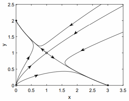
It is of interest to sketch the phase portrait for this nonlinear system. The eigenvectors associated with the unstable saddle point \((1, 1)\) determine the directions of the flow into and away from this fixed point. The eigenvector associated with the positive eigenvalue \(\lambda_1 = −1 +\sqrt{2}\) can be determined from the first equation of \((\mathbf{J}_* − \lambda_1\mathbf{I})\mathbf{v_1 }= 0\), or \[-\sqrt{2}v_{11}-2v_{12}=0,\nonumber\] so that \(v_{12} = −(\sqrt{2}/2)v_{11}\). The eigenvector associated with the negative eigenvalue \(\lambda_1 = −1 −\sqrt{2}\) satisfies \(v_{22} = (\sqrt{2}/2)v_{21}\). The eigenvectors give the slope of the lines with origin at the fixed point for incoming (negative eigenvalue) and outgoing (positive eigenvalue) trajectories. The outgoing trajectories have negative slope \(−\sqrt{2}/2\) and the incoming trajectories have positive slope \(\sqrt{2}/2\). A rough sketch of the phase portrait can be made by hand (as demonstrated in class). Here, a computer generated plot obtained from numerical solution of the nonlinear coupled odes is presented in Fig. \(\PageIndex{1}\). The curve starting from the origin and at infinity, and terminating at the unstable saddle point is called the separatrix. This curve separates the phase space into two regions: initial conditions for which the solution asymptotes to the fixed point \((0, 2)\), and initial conditions for which the solution asymptotes to the fixed point \((3, 0)\).