
8.2: One-Dimensional Bifurcations
- Page ID
- 90429

\( \newcommand{\vecs}[1]{\overset { \scriptstyle \rightharpoonup} {\mathbf{#1}} } \)
\( \newcommand{\vecd}[1]{\overset{-\!-\!\rightharpoonup}{\vphantom{a}\smash {#1}}} \)
\( \newcommand{\dsum}{\displaystyle\sum\limits} \)
\( \newcommand{\dint}{\displaystyle\int\limits} \)
\( \newcommand{\dlim}{\displaystyle\lim\limits} \)
\( \newcommand{\id}{\mathrm{id}}\) \( \newcommand{\Span}{\mathrm{span}}\)
( \newcommand{\kernel}{\mathrm{null}\,}\) \( \newcommand{\range}{\mathrm{range}\,}\)
\( \newcommand{\RealPart}{\mathrm{Re}}\) \( \newcommand{\ImaginaryPart}{\mathrm{Im}}\)
\( \newcommand{\Argument}{\mathrm{Arg}}\) \( \newcommand{\norm}[1]{\| #1 \|}\)
\( \newcommand{\inner}[2]{\langle #1, #2 \rangle}\)
\( \newcommand{\Span}{\mathrm{span}}\)
\( \newcommand{\id}{\mathrm{id}}\)
\( \newcommand{\Span}{\mathrm{span}}\)
\( \newcommand{\kernel}{\mathrm{null}\,}\)
\( \newcommand{\range}{\mathrm{range}\,}\)
\( \newcommand{\RealPart}{\mathrm{Re}}\)
\( \newcommand{\ImaginaryPart}{\mathrm{Im}}\)
\( \newcommand{\Argument}{\mathrm{Arg}}\)
\( \newcommand{\norm}[1]{\| #1 \|}\)
\( \newcommand{\inner}[2]{\langle #1, #2 \rangle}\)
\( \newcommand{\Span}{\mathrm{span}}\) \( \newcommand{\AA}{\unicode[.8,0]{x212B}}\)
\( \newcommand{\vectorA}[1]{\vec{#1}} % arrow\)
\( \newcommand{\vectorAt}[1]{\vec{\text{#1}}} % arrow\)
\( \newcommand{\vectorB}[1]{\overset { \scriptstyle \rightharpoonup} {\mathbf{#1}} } \)
\( \newcommand{\vectorC}[1]{\textbf{#1}} \)
\( \newcommand{\vectorD}[1]{\overrightarrow{#1}} \)
\( \newcommand{\vectorDt}[1]{\overrightarrow{\text{#1}}} \)
\( \newcommand{\vectE}[1]{\overset{-\!-\!\rightharpoonup}{\vphantom{a}\smash{\mathbf {#1}}}} \)
\( \newcommand{\vecs}[1]{\overset { \scriptstyle \rightharpoonup} {\mathbf{#1}} } \)
\(\newcommand{\longvect}{\overrightarrow}\)
\( \newcommand{\vecd}[1]{\overset{-\!-\!\rightharpoonup}{\vphantom{a}\smash {#1}}} \)
\(\newcommand{\avec}{\mathbf a}\) \(\newcommand{\bvec}{\mathbf b}\) \(\newcommand{\cvec}{\mathbf c}\) \(\newcommand{\dvec}{\mathbf d}\) \(\newcommand{\dtil}{\widetilde{\mathbf d}}\) \(\newcommand{\evec}{\mathbf e}\) \(\newcommand{\fvec}{\mathbf f}\) \(\newcommand{\nvec}{\mathbf n}\) \(\newcommand{\pvec}{\mathbf p}\) \(\newcommand{\qvec}{\mathbf q}\) \(\newcommand{\svec}{\mathbf s}\) \(\newcommand{\tvec}{\mathbf t}\) \(\newcommand{\uvec}{\mathbf u}\) \(\newcommand{\vvec}{\mathbf v}\) \(\newcommand{\wvec}{\mathbf w}\) \(\newcommand{\xvec}{\mathbf x}\) \(\newcommand{\yvec}{\mathbf y}\) \(\newcommand{\zvec}{\mathbf z}\) \(\newcommand{\rvec}{\mathbf r}\) \(\newcommand{\mvec}{\mathbf m}\) \(\newcommand{\zerovec}{\mathbf 0}\) \(\newcommand{\onevec}{\mathbf 1}\) \(\newcommand{\real}{\mathbb R}\) \(\newcommand{\twovec}[2]{\left[\begin{array}{r}#1 \\ #2 \end{array}\right]}\) \(\newcommand{\ctwovec}[2]{\left[\begin{array}{c}#1 \\ #2 \end{array}\right]}\) \(\newcommand{\threevec}[3]{\left[\begin{array}{r}#1 \\ #2 \\ #3 \end{array}\right]}\) \(\newcommand{\cthreevec}[3]{\left[\begin{array}{c}#1 \\ #2 \\ #3 \end{array}\right]}\) \(\newcommand{\fourvec}[4]{\left[\begin{array}{r}#1 \\ #2 \\ #3 \\ #4 \end{array}\right]}\) \(\newcommand{\cfourvec}[4]{\left[\begin{array}{c}#1 \\ #2 \\ #3 \\ #4 \end{array}\right]}\) \(\newcommand{\fivevec}[5]{\left[\begin{array}{r}#1 \\ #2 \\ #3 \\ #4 \\ #5 \\ \end{array}\right]}\) \(\newcommand{\cfivevec}[5]{\left[\begin{array}{c}#1 \\ #2 \\ #3 \\ #4 \\ #5 \\ \end{array}\right]}\) \(\newcommand{\mattwo}[4]{\left[\begin{array}{rr}#1 \amp #2 \\ #3 \amp #4 \\ \end{array}\right]}\) \(\newcommand{\laspan}[1]{\text{Span}\{#1\}}\) \(\newcommand{\bcal}{\cal B}\) \(\newcommand{\ccal}{\cal C}\) \(\newcommand{\scal}{\cal S}\) \(\newcommand{\wcal}{\cal W}\) \(\newcommand{\ecal}{\cal E}\) \(\newcommand{\coords}[2]{\left\{#1\right\}_{#2}}\) \(\newcommand{\gray}[1]{\color{gray}{#1}}\) \(\newcommand{\lgray}[1]{\color{lightgray}{#1}}\) \(\newcommand{\rank}{\operatorname{rank}}\) \(\newcommand{\row}{\text{Row}}\) \(\newcommand{\col}{\text{Col}}\) \(\renewcommand{\row}{\text{Row}}\) \(\newcommand{\nul}{\text{Nul}}\) \(\newcommand{\var}{\text{Var}}\) \(\newcommand{\corr}{\text{corr}}\) \(\newcommand{\len}[1]{\left|#1\right|}\) \(\newcommand{\bbar}{\overline{\bvec}}\) \(\newcommand{\bhat}{\widehat{\bvec}}\) \(\newcommand{\bperp}{\bvec^\perp}\) \(\newcommand{\xhat}{\widehat{\xvec}}\) \(\newcommand{\vhat}{\widehat{\vvec}}\) \(\newcommand{\uhat}{\widehat{\uvec}}\) \(\newcommand{\what}{\widehat{\wvec}}\) \(\newcommand{\Sighat}{\widehat{\Sigma}}\) \(\newcommand{\lt}{<}\) \(\newcommand{\gt}{>}\) \(\newcommand{\amp}{&}\) \(\definecolor{fillinmathshade}{gray}{0.9}\)A bifurcation occurs in a nonlinear differential equation when a small change in a parameter results in a qualitative change in the long-time solution. Examples of bifurcations are when fixed points are created or destroyed, or change their stability.
We now consider four classic bifurcations of one-dimensional nonlinear differential equations: saddle-node bifurcation, transcritical bifurcation, supercritical pitchfork bifurcation, and subcritical pitchfork bifurcation. The corresponding differential equation will be written as \[\overset{.}{x}=f_r(x),\nonumber\] where the subscript \(r\) represents a parameter that results in a bifurcation when varied across zero. The simplest differential equations that exhibit these bifurcations are called the normal forms, and correspond to a local analysis (i.e., Taylor series expansion) of more general differential equations around the fixed point, together with a possible rescaling of \(x\).
Saddle-Node Bifurcation
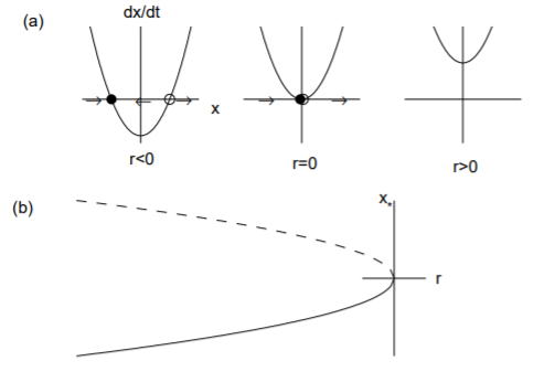
The saddle-node bifurcation results in fixed points being created or destroyed. The normal form for a saddle-node bifurcation is given by \[\overset{.}{x}=r+x^2.\nonumber\]
The fixed points are \(x_* = ±\sqrt{-r}\). Clearly, two real fixed points exist when \(r < 0\) and no real fixed points exist when \(r > 0\). The stability of the fixed points when \(r < 0\) are determined by the derivative of \(f(x) = r + x^2\), given by \(f' (x) = 2x\). Therefore, the negative fixed point is stable and the positive fixed point is unstable.
Graphically, we can illustrate this bifurcation in two ways. First, in Fig. \(\PageIndex{1}\)(a), we plot \(\overset{.}{x}\) versus \(x\) for the three parameter values corresponding to \(r < 0\), \(r = 0\) and \(r > 0\). The values at which \(\overset{.}{x} = 0\) correspond to the fixed points, and arrows are drawn indicating how the solution \(x(t)\) evolves (to the right if \(\overset{.}{x}> 0\) and to the left if \(\overset{.}{x}< 0\)). The stable fixed point is indicated by a filled circle and the unstable fixed point by an open circle. Note that when \(r = 0\), solutions converge to the origin from the left, but diverge from the origin on the right. Second, in Fig. \(\PageIndex{1}\)(b), we plot a bifurcation diagram illustrating the fixed point \(x_*\) versus the bifurcation parameter \(r\). The stable fixed point is denoted by a solid line and the unstable fixed point by a dashed line. Note that the two fixed points collide and annihilate at \(r = 0\), and there are no fixed points for \(r > 0\).
Transcritical Bifurcation
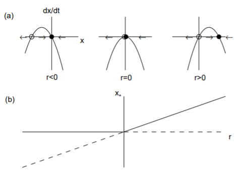
A transcritical bifurcation occurs when there is an exchange of stabilities between two fixed points. The normal form for a transcritical bifurcation is given by \[\overset{.}{x}=rx-x^2.\nonumber\]
The fixed points are \(x_* = 0\) and \(x_* = r\). The derivative of the right-hand-side is \(f' (x) = r − 2x\), so that \(f' (0) = r\) and \(f ' (r) = −r\). Therefore, for \(r < 0\), \(x_* = 0\) is stable and \(x_* = r\) is unstable, while for \(r > 0\), \(x_* = r\) is stable and \(x_* = 0\) is unstable. The two fixed points thus exchange stability as \(r\) passes through zero. The transcritical bifurcation is illustrated in Fig. \(\PageIndex{2}\).
Supercritical Pitchfork Bifurcation
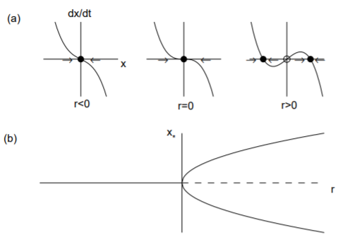
The pitchfork bifurcations occur in physical models where fixed points appear and disappear in pairs due to some intrinsic symmetry of the problem. Pitchfork bifurcations can come in one of two types. In the supercritical bifurcation, a pair of stable fixed points are created at the bifurcation (or critical) point and exist after (super) the bifurcation. In the subcritical bifurcation, a pair of unstable fixed points are created at the bifurcation point and exist before (sub) the bifurcation.
The normal form for the supercritical pitchfork bifurcation is given by \[\overset{.}{x}=rx-x^3.\nonumber\]
Note that the linear term results in exponential growth when \(r > 0\) and the nonlinear term stabilizes this growth. The fixed points are \(x_* = 0\) and \(x_* = ±\sqrt{r}\), the latter fixed points existing only when \(r > 0\). The derivative of \(f\) is \(f' (x) = r − 3x^2\) so that \(f' (0) = r\) and \(f' (±\sqrt{r}) = −2r\). Therefore, the fixed point \(x_* = 0\) is stable for \(r < 0\) and unstable for \(r > 0\) while the fixed points \(x = ±\sqrt{r}\) exist and are stable for \(r > 0\). Notice that the fixed point \(x_* = 0\) becomes unstable as \(r\) crosses zero and two new stable fixed points \(x_* = ±\sqrt{r}\) are born. The supercritical pitchfork bifurcation is illustrated in Fig. \(\PageIndex{3}\).
Supercritical Pitchfork Bifurcation
In the subcritical case, the cubic term is destabilizing. The normal form (to order \(x^3\)) is \[\overset{.}{x}=rx+x^3.\nonumber\]
The fixed points are \(x_* = 0\) and \(x_* = ±\sqrt{-r}\), the latter fixed points existing only when \(r ≤ 0\). The derivative of the right-hand-side is \(f' (x) = r +3x^2\) so that \(f' (0) = r\) and \(f' (±\sqrt{-r}) = −2r\). Therefore, the fixed point \(x_* = 0\) is stable for \(r < 0\) and unstable for \(r > 0\) while the fixed points \(x = ±\sqrt{-r}\) exist and are unstable for \(r < 0\). There are no stable fixed points when \(r > 0\).
The absence of stable fixed points for \(r > 0\) indicates that the neglect of terms of higher-order in \(x\) than \(x^3\) in the normal form may be unwarranted. Keeping to the intrinsic symmetry of the equations (only odd powers of \(x\)) we can add a stabilizing nonlinear term proportional to \(x^5\). The extended normal form (to order \(x^5\)) is \[\overset{.}{x}=rx+x^3-x^5,\nonumber\] and is somewhat more difficult to analyze. The fixed points are solutions of \[x(r+x^2-x^4)=0.\nonumber\]
The fixed point \(x_* = 0\) exists for all \(r\), and four additional fixed points can be found from the solutions of the quadratic equation in \(x^2\):
\[x_*=\pm\sqrt{\frac{1}{2}(1\pm\sqrt{1+4r})}.\nonumber\]
These fixed points exist only if \(x_*\) is real. Clearly, for the inner square-root to be real, \(r ≥ −1/4\). Also observe that \(1 −\sqrt{1+4r}\) becomes negative for \(r > 0\). We thus have three intervals in \(r\) to consider, and these regions and their fixed points are \[\begin{array}{rlll} r<-\frac{1}{4}: & x_*=0 &\text{(one fixed point);} \\ -\frac{1}{4}<r<0: & x_*=0, &x_*=\pm\sqrt{\frac{1}{2}(1\pm\sqrt{1+4r})} &\text{(five fixed points);} \\ r>0: &x_*=0, &x_*=\pm\sqrt{\frac{1}{2}(1+\sqrt{1+4r})} &\text{(three fixed points).}\end{array}\nonumber\]
Stability is determined from \(f' (x) = r + 3x^2 − 5x^4\). Now, \(f' (0) = r\) so \(x_* = 0\) is stable for \(r < 0\) and unstable for \(r > 0\). The calculation for the other four roots can be simplified by noting that \(x_*\) satisfies \(r + x_*^2 − x_*^4 = 0\), or \(x_*^4 = r + x_*^2\). Therefore, \[\begin{aligned}f'(x_*)&=r+3x_*^2-5x_*^4 \\ &=r+3x_*^2-5(r+x_*^2) \\ &=-4r-2x_*^2 \\ &=-2(2r+x_*^2).\end{aligned}\]
With \(x_*^2=\frac{1}{2}(1\pm\sqrt{1+4r})\), we have \[\begin{aligned} f'(x_*)&=-2\left(2r+\frac{1}{2}(1\pm\sqrt{1+4r})\right) \\ &=-\left( (1+4r)\pm\sqrt{1+4r}\right) \\ &=-\sqrt{1+4r}\left(\sqrt{1+4r}\pm 1\right).\end{aligned}\]
Clearly, the plus root is always stable since \(f' (x_*) < 0\). The minus root exists only for \(−\frac{1}{4}< r < 0\) and is unstable since \(f' (x_*) > 0\). We summarize the stability of the various fixed points:
\[\begin{array}{rll} r<-\frac{1}{4}:&x_*=0&\text{(stable);} \\ -\frac{1}{4}<r<0:&x_*=0,&\text{(stable)} \\ &x_*=\pm\sqrt{\frac{1}{2}(1+\sqrt{1+4r})}&\text{(stable);} \\ &x_*=\pm\sqrt{\frac{1}{2}(1-\sqrt{1+4r})}&\text{(unstable);} \\ r>0:&x_*=0&\text{(unstable)} \\ &x_*=\pm\sqrt{\frac{1}{2}(1+\sqrt{1+4r})}&\text{(stable).}\end{array}\nonumber\]
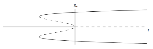
The bifurcation diagram is shown in Fig. \(\PageIndex{4}\), and consists of a subcritical pitchfork bifurcation at \(r = 0\) and two saddle-node bifurcations at \(r = −1/4\). We can imagine what happens to \(x\) as \(r\) increases from negative values, supposing there is some small noise in the system so that \(x = x(t)\) will diverge from unstable fixed points. For \(r < −1/4\), the equilibrium value of \(x\) is \(x_* = 0\). As \(r\) increases into the range \(−1/4 < r < 0\), \(x\) will remain at \(x_* = 0\). However, a catastrophe occurs as soon as \(r > 0\). The \(x_* = 0\) fixed point becomes unstable and the solution will jump up (or down) to the only remaining stable fixed point. Such behavior is called a jump bifurcation. A similar catastrophe can happen as \(r\) decreases from positive values. In this case, the jump occurs as soon as \(r < −1/4\).
Since the stable equilibrium value of \(x\) depends on whether we are increasing or decreasing \(r\), we say that the system exhibits hysteresis. The existence of a subcritical pitchfork bifurcation can be very dangerous in engineering applications since a small change in a problem’s parameters can result in a large change in the equilibrium state. Physically, this can correspond to a collapse of a structure, or the failure of a component.