1.2: Linear Constant Coefficient Equations

Let’s consider the linear first order constant coefficient partial differential equation

\[\label{eq:1}au_x+bu_y+cu=f(x,y), \]

for \(a,\: b,\) and \(c\) constants with \(a^2 + b^2 > 0\). We will consider how such equations might be solved. We do this by considering two cases, \(b = 0\) and \(b\neq 0\).

Integrating this equation and solving for \(u(x, y)\), we have

\[\begin{align}\mu (x)u(x,y)&=\frac{1}{a}\int f(\xi ,y)\mu (\xi )d\xi +g(y) \nonumber \\ e^{\frac{c}{a}x}u(x,y)&=\frac{1}{a}\int f(\xi ,y)e^{\frac{c}{a}\xi}d\xi +g(y)\nonumber \\ u(x,y)&=\frac{1}{a}\int f(\xi ,y)e^{\frac{c}{a}(\xi -x)}d\xi +g(y)e^{-\frac{c}{a}x}.\label{eq:2}\end{align} \]

Here \(g(y)\) is an arbitrary function of \(y\).

For the second case, \(b\neq 0\), we have to solve the equation

\[au_x+bu_y+cu=f.\nonumber \]

It would help if we could find a transformation which would eliminate one of the derivative terms reducing this problem to the previous case. That is what we will do.

We first note that

\[\begin{align}au_x+bu_y&=(a\mathbf{i}+b\mathbf{j})\cdot (u_x\mathbf{i}+u_y\mathbf{j})\nonumber \\ &=(a\mathbf{i}+b\mathbf{j})\cdot\nabla u.\label{eq:3}\end{align} \]

Recall from multivariable calculus that the last term is nothing but a directional derivative of \(u(x, y)\) in the direction \(a\mathbf{i} + b\mathbf{j}\). [Actually, it is proportional to the directional derivative if \(a\mathbf{i} + b\mathbf{j}\) is not a unit vector.]

Figure \(\PageIndex{1}\): Coordinate systems for transforming \(au_x + bu_y + cu = f\) into \(bv_z + cv = f\) using the transformation \(w = bx − ay\) and \(z = y\).

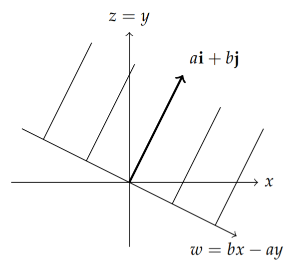
Therefore, we seek to write the partial differential equation as involving a derivative in the direction \(a\mathbf{i} + b\mathbf{j}\) but not in a directional orthogonal to this. In Figure \(\PageIndex{1}\) we depict a new set of coordinates in which the \(w\) direction is orthogonal to \(a\mathbf{i} + b\mathbf{j}\).

We consider the transformation

\[\begin{align}w&=bx-ay, \nonumber \\ z&=y.\label{eq:4}\end{align} \]

We first note that this transformation is invertible,

\[\begin{align} x&=\frac{1}{b}(w+az), \nonumber \\ y&=z.\label{eq:5}\end{align} \]

Next we consider how the derivative terms transform. Let \(u(x, y) = v(w, z)\). Then, we have

\[\begin{align}au_x+bu_y&=a\frac{\partial}{\partial x}v(w,z)+b\frac{\partial}{\partial y}v(w,z),\nonumber \\ &=a\left[\frac{\partial v}{\partial w}\frac{\partial w}{\partial x}+\frac{\partial v}{\partial z}\frac{\partial z}{\partial x}\right] \nonumber \\ &\: +b\left[\frac{\partial v}{\partial w}\frac{\partial w}{\partial y}+\frac{\partial v}{\partial z}\frac{\partial z}{\partial y}\right] \nonumber \\ &=a[bv_w+0\cdot v_z]+b[-av_w+v_z]\nonumber \\ &=bv_z.\label{eq:6}\end{align} \]

Therefore, the partial differential equation becomes

\[bv_z+cv=f\left(\frac{1}{b}(w+az),z\right).\nonumber \]

This is now in the same form as in the first case and can be solved using an integrating factor.

Example \(\PageIndex{1}\)

Find the general solution of the equation \(3u_x − 2u_y + u = x\).

Solution

First, we transform the equation into new coordinates.

\[w=bx-ay=-2x-3y,\nonumber \]

and \(z=y\). The,

\[\begin{align}u_x-2u_y&=3[-2v_w+0\cdot v_z]-2[-3v_w+v_z] \nonumber \\ &=-2v_z.\label{eq:7}\end{align} \]

Using this integrating factor, we can solve the differential equation for \(v(w, z)\).

\[\begin{align}\frac{\partial}{\partial z}\left(e^{-z/2}v\right)&=\frac{1}{4}(w+3z)e^{-z/2},\nonumber \\ e^{-z/2}v(w,z)&=\frac{1}{4}\int^z (w+3\xi )e^{-\xi /2}d\xi \nonumber \\ &=-\frac{1}{2}(w+6+3z)e^{-z/2}+c(w) \nonumber \\ v(w,z)&=-\frac{1}{2}(w+6+3z)+c(w)e^{z/2}\nonumber \\ u(x,y)&=x-3+c(-2x-3y)e^{y/2}.\label{eq:8}\end{align} \]