1.3: Quasilinear Equations - The Method of Characteristics

Geometric Interpretation

We consider the quasilinear partial differential equation in two independent variables,

\[\label{eq:1}a(x,y,u)u_x+b(x,y,u)u_y-c(x,y,u)=0. \]

Let \(u = u(x, y)\) be a solution of this equation. Then,

\[f(x,y,u)=u(x,y)-u=0\nonumber \]

describes the solution surface, or integral surface.

We recall from multivariable, or vector, calculus that the normal to the integral surface is given by the gradient function,

\[\nabla f=(u_x, u_y, -1).\nonumber \]

Now consider the vector of coefficients, \(\mathbf{v} = (a, b, c)\) and the dot product with the gradient above:

\[\mathbf{v}\cdot\nabla f=au_x+bu_y-c.\nonumber \]

This is the left hand side of the partial differential equation. Therefore, for the solution surface we have

\[\mathbf{v}\cdot\nabla f=0,\nonumber \]

or \(\mathbf{v}\) is perpendicular to \(\nabla f\). Since \(\nabla f\) is normal to the surface, \(\mathbf{v} = (a, b, c)\) is tangent to the surface. Geometrically, \(\mathbf{v}\) defines a direction field, called the characteristic field. These are shown in Figure \(\PageIndex{1}\).

Characteristics

We seek the forms of the characteristic curves such as the one shown in Figure \(\PageIndex{1}\). Recall that one can parametrize space curves,

\[\mathbf{c}(t)=(x(t),y(t),u(t)),\quad t∈ [t_1 , t_2].\nonumber \]

The tangent to the curve is then

\[\mathbf{v}(t)=\frac{d\mathbf{c}(t)}{dt}=\left(\frac{dx}{dt},\frac{dy}{dt}, \frac{du}{dt}\right).\nonumber \]

However, in the last section we saw that \(\mathbf{v}(t) = (a, b, c)\) for the partial differential equation \(a(x, y, u)u_x + b(x, y, u)u_y − c(x, y, u) = 0\). This gives the parametric form of the characteristic curves as

\[\label{eq:2}\frac{dx}{dt}=a,\quad\frac{dy}{dt}=b,\quad\frac{du}{dt}=c. \]

Another form of these equations is found by relating the differentials, \(dx,\: dy,\: du\), to the coefficients in the differential equation. Since \(x = x(t)\) and \(y = y(t)\), we have

\[\frac{dy}{dx}=\frac{dy/dt}{dx/dt}=\frac{b}{a}.\nonumber \]

Similarly, we can show that

\[\frac{du}{dx}=\frac{c}{a},\quad\frac{du}{dy}=\frac{c}{b}.\nonumber \]

All of these relations can be summarized in the form

\[\label{eq:3}dt=\frac{dx}{a}=\frac{dy}{b}=\frac{du}{c}. \]

How do we use these characteristics to solve quasilinear partial differential equations? Consider the next example.

Example \(\PageIndex{1}\)

Find the general solution: \(u_x + u_y − u = 0\).

Solution

We first identify \(a = 1,\: b = 1,\) and \(c = u\). The relations between the differentials is

\[\frac{dx}{1}=\frac{dy}{1}=\frac{du}{u}.\nonumber \]

We can pair the differentials in three ways:

\[\frac{dy}{dx}=1,\quad\frac{du}{dx}=u,\quad\frac{du}{dy}=u.\nonumber \]

Only two of these relations are independent. We focus on the first pair.

The first equation gives the characteristic curves in the xy-plane. This equation is easily solved to give

\[y=x+c_1.\nonumber \]

The second equation can be solved to give \(u=c_2e^x\).

The goal is to find the general solution to the differential equation. Since \(u = u(x, y)\), the integration “constant” is not really a constant, but is constant with respect to \(x\). It is in fact an arbitrary constant function. In fact, we could view it as a function of \(c_1\), the constant of integration in the first equation. Thus, we let \(c_2 = G(c_1)\) for \(G\) and arbitrary function. Since \(c_1 = y − x\), we can write the general solution of the differential equation as

\[u(x,y)=G(y-x)e^x .\nonumber \]

Example \(\PageIndex{2}\)

Solve the advection equation, \(u_t + cu_x = 0\), for \(c\) a constant, and \(u = u(x, t)\), \(|x| < \infty\), \(t > 0\).

Solution

The characteristic equations are

\[\label{eq:4}d\tau =\frac{dt}{1}=\frac{dx}{c}=\frac{du}{0} \]

and the parametric equations are given by

\[\label{eq:5}\frac{dx}{d\tau}=c,\quad\frac{du}{d\tau}=0. \]

These equations imply that

• \(u=\text{const.}=c_1\).
• \(x=ct+\text{const.}=ct+c_2\).

As before, we can write \(c_1\) as an arbitrary function of \(c_2\). However, before doing so, let’s replace \(c_1\) with the variable \(\xi\) and then we have that

\[\xi =x-ct,\quad u(x,t)=f(\xi )=f(x-ct)\nonumber \]

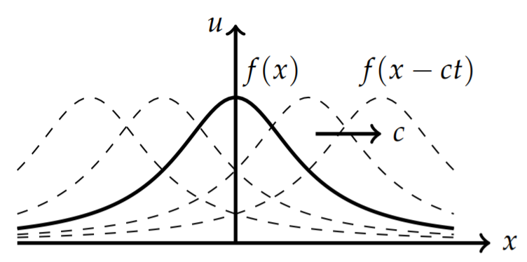
where \(f\) is an arbitrary function. Furthermore, we see that \(u(x, t) = f(x − ct)\) indicates that the solution is a wave moving in one direction in the shape of the initial function, \(f(x)\). This is known as a traveling wave. A typical traveling wave is shown in Figure \(\PageIndex{2}\).

Figure \(\PageIndex{2}\): Depiction of a traveling wave. \(u(x, t) = f(x)\) at \(t = 0\) travels without changing shape.

Note that since \(u = u(x, t)\), we have

\[\begin{align}0&=u_t+cu_x\nonumber \\ &=\frac{\partial u}{\partial t}+\frac{dx}{dt}\frac{\partial u}{\partial x}\nonumber \\ &=\frac{du(x(t),t}{dt}.\label{eq:6}\end{align} \]

This implies that \(u(x, t) =\) constant along the characteristics, \(\frac{dx}{dt} = c\).

As with ordinary differential equations, the general solution provides an infinite number of solutions of the differential equation. If we want to pick out a particular solution, we need to specify some side conditions. We investigate this by way of examples.

Example \(\PageIndex{3}\)

Find solutions of \(u_x + u_y − u = 0\) subject to \(u(x, 0) = 1\).

Solution

We found the general solution to the partial differential equation as \(u(x, y) = G(y − x)e^x\). The side condition tells us that \(u = 1\) along \(y = 0\). This requires

\[1=u(x,0)=G(-x)e^x.\nonumber \]

Thus, \(G(−x) = e^{−x}\). Replacing \(x\) with \(−z\), we find

\[G(z)=e^z.\nonumber \]

Thus, the side condition has allowed for the determination of the arbitrary function \(G(y − x)\). Inserting this function, we have

\[u(x,y)=G(y-x)e^x=e^{y-x}e^x=e^y.\nonumber \]

Side conditions could be placed on other curves. For the general line, \(y = mx + d\), we have \(u(x, mx + d) = g(x)\) and for \(x = d\), \(u(d, y) = g(y)\). As we will see, it is possible that a given side condition may not yield a solution. We will see that conditions have to be given on non-characteristic curves in order to be useful.

Example \(\PageIndex{4}\)

Find solutions of \(3u_x − 2u_y + u = x\) for

1. \(u(x, x) = x\) and
2. \(u(x, y) = 0\) on \(3y + 2x = 1\).

Solution

Before applying the side condition, we find the general solution of the partial differential equation. Rewriting the differential equation in standard form, we have

\[3u_x-2u_y=x=u.\nonumber \]

The characteristic equations are

\[\label{eq:7}\frac{dx}{3}=\frac{dy}{-2}=\frac{du}{x-u}. \]

These equations imply that

• \(-2dx=3dy\)
  This implies that the characteristic curves (lines) are \(2x + 3y = c_1\).
• \(\frac{du}{dx}=\frac{1}{3}(x-u).\)
  This is a linear first order differential equation, \(\frac{du}{dx} + \frac{1}{3}u = \frac{1}{3}x\). It can be solved using the integrating factor,

  \[\mu (x)=\exp\left(\frac{1}{3}\int^x d\xi\right)=e^{x/3}.\nonumber \]

  \[\begin{align}\frac{d}{dx}\left(ue^{x/3}\right)&=\frac{1}{3}xe^{x/3}\nonumber \\ ue^{x/3}&=\frac{1}{3}\int^x \xi e^{\xi /3}d\xi +c_2 \nonumber \\ &=(x-3)e^{x/3}+c_2\nonumber \\ u(x,y)&=x-3+c_2e^{-x/3}.\label{eq:8}\end{align} \]

As before, we write \(c_2\) as an arbitrary function of \(c_1 = 2x + 3y\). This gives the general solution

\[u(x,y)=x-3+G(2x+3y)e^{-x/3}.\nonumber \]

Note that this is the same answer that we had found in Example 1.1.1

Now we can look at any side conditions and use them to determine particular solutions by picking out specific \(G\)’s.

1. \(u(x,x)=x\)
   This states that \(u = x\) along the line \(y = x\). Inserting this condition into the general solution, we have

   \[x=x-3+G(5x)e^{-x/3},\nonumber \]

   or

   \[G(5x)=3e^{x/3}.\nonumber \]

   Letting \(z = 5x\),

   \[G(z)=3e^{z/15}.\nonumber \]

   

   Figure \(\PageIndex{3}\): Integral surface found in Example \(\PageIndex{4}\)

   The particular solution satisfying this side condition is

   \[\begin{align}u(x,y)&=x-3+G(2x+3y)e^{-x/3}\nonumber \\ &=x-3+3e^{(2x+3y)/15}e^{-x/3}\nonumber \\ &=x-3+3e^{(y-x)/5}.\label{eq:9}\end{align} \]

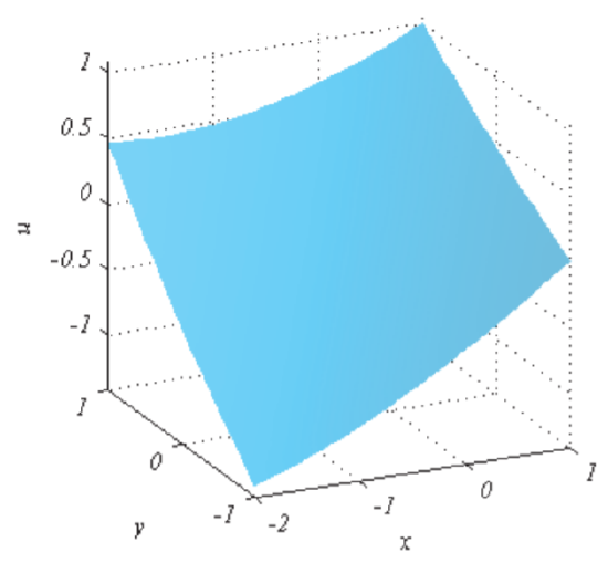
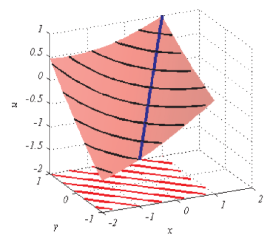
   This surface is shown in Figure \(\PageIndex{4}\).

   

   Figure \(\PageIndex{4}\): Integral surface with side condition and characteristics for Example \(\PageIndex{4}\).

   In Figure \(\PageIndex{4}\) we superimpose the values of \(u(x, y)\) along the characteristic curves. The characteristic curves are the red lines and the images of these curves are the black lines. The side condition is indicated with the blue curve drawn along the surface.
   The values of \(u(x, y)\) are found from the side condition as follows. For \(x =\xi\) on the blue curve, we know that \(y =\xi\) and \(u(\xi , \xi ) =\xi\). Now, the characteristic lines are given by \(2x + 3y = c_1\). The constant \(c_1\) is found on the blue curve from the point of intersection with one of the black characteristic lines. For \(x = y =\xi\), we have \(c_1 = 5\xi\). Then, the equation of the characteristic line, which is red in Figure \(\PageIndex{4}\), is given by \(y = \frac{1}{3}(5\xi − 2x)\).
   Along these lines we need to find \(u(x, y) = x − 3 + c_2e^{−x/3}\). First we have to find \(c_2\). We have on the blue curve, that

   \[\begin{align}\xi&=u(\xi,\xi)\nonumber \\ &=\xi -3+c_2e^{-\xi /3}.\label{eq:10}\end{align} \]

   Therefore, \(c_2 = 3e^{\xi /3}\). Inserting this result into the expression for the solution, we have

   \[u(x,y)=x-3+e^{(\xi -x)/3}.\nonumber \]

   So, for each \(\xi\), one can draw a family of spacecurves

   \[\left(x,\: \frac{1}{3}(5\xi -2x),\: x-3+e^{(\xi -x)/3}\right)\nonumber \]

   yielding the integral surface.

2. \(u(x,y)=0\) on \(3y+2x=1\).
   For this condition, we have

   \[0=x-3+G(1)e^{-x/3}.\nonumber \]

   We note that \(G\) is not a function in this expression. We only have one value for \(G\). So, we cannot solve for \(G(x)\). Geometrically, this side condition corresponds to one of the black curves in Figure \(\PageIndex{4}\).