
2.5: Laplace’s Equation in 2D


- Last updated
- Sep 4, 2024
- Save as PDF

( \newcommand{\kernel}{\mathrm{null}\,}\)
Another generic partial differential equation is Laplace’s equation, ∇2u=0. Laplace’s equation arises in many applications. As an example, consider a thin rectangular plate with boundaries set at fixed temperatures. Assume that any temperature changes of the plate are governed by the heat equation, ut=k∇2u, subject to these boundary conditions. However, after a long period of time the plate may reach thermal equilibrium. If the boundary temperature is zero, then the plate temperature decays to zero across the plate. However, if the boundaries are maintained at a fixed nonzero temperature, which means energy is being put into the system to maintain the boundary conditions, the internal temperature may reach a nonzero equilibrium temperature. Reaching thermal equilibrium means that asymptotically in time the solution becomes time independent. Thus, the equilibrium state is a solution of the time independent heat equation, ∇2u=0.
A second example comes from electrostatics. Letting ϕ(r) be the electric potential, one has for a static charge distribution, ρ(r), that the electric field, E=∇ϕ, satisfies one of Maxwell’s equations, ∇·E=ρ/ϵ0. In regions devoid of charge, ρ(r)=0, the electric potential satisfies Laplace’s equation, ∇2ϕ=0.
As a final example, Laplace’s equation appears in two-dimensional fluid flow. For an incompressible flow, ∇·v=0. If the flow is irrotational, then ∇×v=0. We can introduce a velocity potential, v=∇ϕ. Thus, ∇×v vanishes by a vector identity and ∇·v=0 implies ∇2ϕ=0. So, once again we obtain Laplace’s equation.
Solutions of Laplace’s equation are called harmonic functions and we will encounter these in Chapter 8 on complex variables and in Section 2.5 we will apply complex variable techniques to solve the two-dimensional Laplace equation. In this section we use the Method of Separation of Variables to solve simple examples of Laplace’s equation in two dimensions. Three dimensional problems will studied in Chapter 6.
Let’s consider Laplace’s equation in Cartesian coordinates,
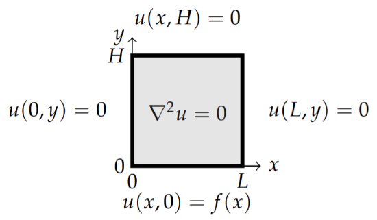
uxx+uyy=0,0<x<L,0<y<H
with the boundary conditions
u(0,y)=0,u(L,y)=0,u(x,0)=f(x),u(x,H)=0.
The boundary conditions are shown in Figure 2.5.1.
Solution
As with the heat and wave equations, we can solve this problem using the method of separation of variables. Let u(x,y)=X(x)Y(y). Then, Laplace’s equation becomes
X″Y+XY″=0
and we can separate the x and y dependent functions and introduce a separation constant, λ,
X″X=−Y″Y=−λ.
Thus, we are led to two differential equations,
X″+λX=0,Y″−λY=0.
The general solution of the equation for Y(y) is given by
Y(y)=c1e√λy+c2e−√λy.
The boundary condition u(x,H)=0 implies Y(H)=0. So, we have
c1e√λH+c2e−√λH=0.
Thus,
c2=−c1e2√λH.
Inserting this result into the expression for Y(y), we have
Y(y)=c1e√λy−c1e2√λHe−√λy=c1e√λH(e−√λHe√λy−e√λHe−√λy)=c1e√λH(e−√λ(H−y)−e√λ(H−y))=−2c1e√λHsinh√λ(H−y).
Since we already know the values of the eigenvalues λn from the eigenvalue problem for X(x), we have that the y-dependence is given by
Yn(y)=sinhnπ(H−y)L.
So, the product solutions are given by
un(x,y)=sinnπxLsinhnπ(H−y)L,n=1,2,….
These solutions satisfy Laplace’s equation and the three homogeneous boundary conditions and in the problem.
The remaining boundary condition, u(x,0)=f(x), still needs to be satisfied. Inserting y=0 in the product solutions does not satisfy the boundary condition unless f(x) is proportional to one of the eigenfunctions Xn(x). So, we first write down the general solution as a linear combination of the product solutions,
u(x,y)=∞∑n=1ansinnπxLsinhnπ(H−y)L.
Now we apply the boundary condition, u(x,0)=f(x), to find that
f(x)=∞∑n=1ansinhnπHLsinnπxL.
Defining bn=ansinhnπHL, this becomes
f(x)=∞∑n=1bnsinnπxL.
We see that the determination of the unknown coefficients, bn, is simply done by recognizing that this is a Fourier sine series. We now move on to the study of Fourier series and provide more complete answers in Chapter 6.