6.5: Laplace’s Equation and Spherical Symmetry


- Last updated
- Sep 4, 2024
- Save as PDF

( \newcommand{\kernel}{\mathrm{null}\,}\)
We have seen that Laplace's equation, ∇2u=0, arises in electrostatics as an equation for electric potential outside a charge distribution and it occurs as the equation governing equilibrium temperature distributions. As we had seen in the last chapter, Laplace’s equation generally occurs in the study of potential theory, which also includes the study of gravitational and fluid potentials. The equation is named after Pierre-Simon Laplace (1749-1827) who had studied the properties of this equation. Solutions of Laplace’s equation are called harmonic functions.
Solve Laplace’s equation in spherical coordinates.
Solution
We seek solutions of this equation inside a sphere of radius r subject to the boundary condition as shown in Figure 6.5.1. The problem is given by Laplace’s equation Laplace’s equation in spherical coordinates1
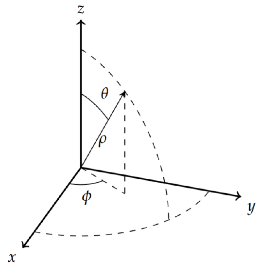
1ρ2∂∂ρ(ρ2∂u∂ρ)+1ρ2sinθ∂∂θ(sinθ∂u∂θ)+1ρ2sin2θ∂2u∂ϕ2=0,
where u=u(ρ,θ,ϕ).
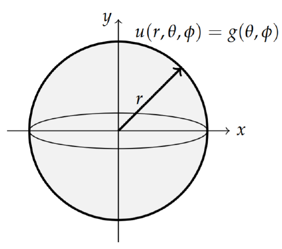
The boundary conditions are given by
u(r,θ,ϕ)=g(θ,ϕ),0<ϕ<2π,0<θ<π,
and the periodic boundary conditions
u(ρ,θ,0)=u(ρ,θ,2π),uϕ(ρ,θ,0)=uϕ(ρ,θ,2π),
where 0<ρ<∞, and 0<θ<π.
The Laplacian in spherical coordinates is given in Problem ?? in Chapter 8.
As before, we perform a separation of variables by seeking product solutions of the form u(ρ,θ,ϕ)=R(ρ)Θ(θ)Φ(ϕ). Inserting this form into the Laplace equation, we obtain
ΘΦρ2ddρ(ρ2dRdρ)+RΦρ2sinθddθ(sinθdΘdθ)+RΘρ2sin2θd2Φdϕ2=0.
Multiplying this equation by ρ2 and dividing by RΘΦ, yields
1Rddρ(ρ2dRdρ)+1sinθΘddθ(sinθdΘdθ)+1sin2θΦd2Φdϕ2=0.
Note that the first term is the only term depending upon ρ. Thus, we can separate out the radial part. However, there is still more work to do on the other two terms, which give the angular dependence. Thus, we have
−1Rddρ(ρ2dRdρ)=1sinθΘddθ(sinθdΘdθ)+1sin2θΦd2Φdϕ2=−λ,
where we have introduced the first separation constant. This leads to two equations:
ddρ(ρ2dRdρ)−λR=0
and
1sinθΘddθ(sinθdΘdθ)+1sin2θΦd2Φdϕ2=−λ.
The final separation can be performed by multiplying the last equation by sin2θ, rearranging the terms, and introducing a second separation constant:
sinθΘddθ(sinθdΘdθ)+λsin2θ=−1Φd2Φdϕ2=μ.
From this expression we can determine the differential equations satisfied by Θ(θ) and Φ(ϕ) :
sinθddθ(sinθdΘdθ)+(λsin2θ−μ)Θ=0
and
d2Φdϕ2+μΦ=0.
Equation (???) is a key equation which occurs when studying problems possessing spherical symmetry. It is an eigenvalue problem for Y(θ,ϕ)=Θ(θ)Φ(ϕ), LY=−λY, where
L=1sinθ∂∂θ(sinθ∂∂θ)+1sin2θ∂2∂ϕ2.
The eigenfunctions of this operator are referred to as spherical harmonics.
We now have three ordinary differential equations to solve. These are the radial equation (???) and the two angular equations (???)-(???). We note that all three are in Sturm-Liouville form. We will solve each eigenvalue problem subject to appropriate boundary conditions.
The simplest of these differential equations is Equation (???) for Φ(ϕ). We have seen equations of this form many times and the general solution is a linear combination of sines and cosines. Furthermore, in this problem u(ρ,θ,ϕ) is periodic in ϕ,
u(ρ,θ,0)=u(ρ,θ,2π),uϕ(ρ,θ,0)=uϕ(ρ,θ,2π).
Since these conditions hold for all ρ and θ, we must require that Φ(ϕ) satisfy the periodic boundary conditions
Φ(0)=Φ(2π),Φ′(0)=Φ′(2π).
The eigenfunctions and eigenvalues for Equation (???) are then found as
Φ(ϕ)={cosmϕ,sinmϕ},μ=m2,m=0,1,….
Next we turn to solving equation, (???). We first transform this equation in order to identify the solutions. Let x=cosθ. Then the derivatives with respect to θ transform as
ddθ=dxdθddx=−sinθddx.
Letting y(x)=Θ(θ) and noting that sin2θ=1−x2, Equation (???) becomes
ddx((1−x2)dydx)+(λ−m21−x2)y=0.
We further note that x∈[−1,1], as can be easily confirmed by the reader.
This is a Sturm-Liouville eigenvalue problem. The solutions consist of a set of orthogonal eigenfunctions. For the special case that m=0 Equation (???) becomes
ddx((1−x2)dydx)+λy=0.
In a course in differential equations one learns to seek solutions of this equation in the form
y(x)=∞∑n=0anxn.
This leads to the recursion relation
an+2=n(n+1)−λ(n+2)(n+1)an.
Setting n=0 and seeking a series solution, one finds that the resulting series does not converge for x=±1. This is remedied by choosing λ=ℓ(ℓ+1) for ℓ=0,1,…, leading to the differential equation
ddx((1−x2)dydx)+ℓ(ℓ+1)y=0.
We saw this equation in Chapter 5 in the form
(1−x2)y′′−2xy′+ℓ(ℓ+1)y=0.
The solutions of this differential equation are Legendre polynomials, denoted by Pℓ(x)
For the more general case, m≠0, the differential equation (???) with λ=ℓ(ℓ+1) becomes
ddx((1−x2)dydx)+(ℓ(ℓ+1)−m21−x2)y=0.
The solutions of this equation are called the associated Legendre functions. The two linearly independent solutions are denoted by Pmℓ(x) and Qmℓ(x). The latter functions are not well behaved at x=±1, corresponding to the north and south poles of the original problem. So, we can throw out these solutions in many physical cases, leaving
Θ(θ)=Pmℓ(cosθ)
as the needed solutions. In Table 6.5 we list a few of these.
| Pmn(x) | Pmn(cosθ) | |
|---|---|---|
| P00(x) | 1 | 1 |
| P01(x) | x | cosθ |
| P11(x) | −(1−x2)12 | −sinθ |
| P02(x) | 12(3x2−1) | 12(3cos2θ−1) |
| P12(x) | −3x(1−x2)12 | −3cosθsinθ |
| P22(x) | 3(1−x2) | 3sin2θ |
| P03(x) | 12(5x3−3x) | 12(5cos3θ−3cosθ) |
| P13(x) | −32(5x2−1)(1−x2)12 | −32(5cos2θ−1)sinθ |
| P23(x) | 15x(1−x2) | 15cosθsin2θ |
| P33(x) | −15(1−x2)32 | −15sin3θ |
The associated Legendre functions are related to the Legendre polynomials by2
Pmℓ(x)=(−1)m(1−x2)m/2dmdxmPℓ(x),
for ℓ=0,1,2,… and m=0,1,…,ℓ. We further note that P0ℓ(x)=Pℓ(x), as one can see in the table. Since Pℓ(x) is a polynomial of degree ℓ, then for m>ℓ,dmdxmPℓ(x)=0 and Pmℓ(x)=0.
Furthermore, since the differential equation only depends on m2,P−mℓ(x) is proportional to Pmℓ(x). One normalization is given by
P−mℓ(x)=(−1)m(ℓ−m)!(ℓ+m)!Pmℓ(x).
The associated Legendre functions also satisfy the orthogonality condition
∫1−1Pmℓ(x)Pmℓ′(x)dx=22ℓ+1(ℓ+m)!(ℓ−m)!δℓℓ′.
The last differential equation we need to solve is the radial equation. With λ=ℓ(ℓ+1),ℓ=0,1,2,…, the radial equation (???) can be written as
ρ2R′′+2ρR′−ℓ(ℓ+1)R=0.
The radial equation is a Cauchy-Euler type of equation. So, we can guess the form of the solution to be R(ρ)=ρs, where s is a yet to be determined constant. Inserting this guess into the radial equation, we obtain the characteristic equation
s(s+1)=ℓ(ℓ+1).
Solving for s, we have
s=ℓ,−(ℓ+1).
Thus, the general solution of the radial equation is
R(ρ)=aρℓ+bρ−(ℓ+1).
We would normally apply boundary conditions at this point. The boundary condition u(r,θ,ϕ)=g(θ,ϕ) is not a homogeneous boundary condition, so we will need to hold off using it until we have the general solution to the three dimensional problem. However, we do have a hidden condition. Since we are interested in solutions inside the sphere, we need to consider what happens at ρ=0. Note that ρ−(ℓ+1) is not defined at the origin. Since the solution is expected to be bounded at the origin, we can set b=0. So, in the current problem we have established that
R(ρ)=aρℓ.
When seeking solutions outside the sphere, one considers the boundary condition R(ρ)→0 as ρ→∞. In this case, R(ρ)=ρ−(ℓ+1).
We have carried out the full separation of Laplace’s equation in spherical coordinates. The product solutions consist of the forms
u(ρ,θ,ϕ)=ρℓPmℓ(cosθ)cosmϕ
and
u(ρ,θ,ϕ)=ρℓPmℓ(cosθ)sinmϕ
for ℓ=0,1,2,… and m=0,±1,…,±ℓ. These solutions can be combined to give a complex representation of the product solutions as
u(ρ,θ,ϕ)=ρℓPmℓ(cosθ)eimϕ.
The general solution is then given as a linear combination of these product can be rewritten as solutions. As there are two indices, we have a double sum:3
u(ρ,θ,ϕ)=∞∑ℓ=0ℓ∑m=−ℓaℓmρℓPmℓ(cosθ)eimϕ.
While this appears to be a complex-valued solution, it can be rewritten as a sum over real functions. The inner sum contains terms for both m=k and to give a complex representation of the product solutions as m=−k. Adding these contributions, we have that
aℓkρℓPkℓ(cosθ)eikϕ+aℓ(−k)ρℓP−kℓ(cosθ)e−ikϕ
can be rewritten as
(Aℓkcoskϕ+Bℓksinkϕ)ρℓPkℓ(cosθ).
As a simple example we consider the solution of Laplace’s equation in which there is azimuthal symmetry. Let
u(r,θ,ϕ)=g(θ)=1−cos2θ.
This function is zero at the poles and has a maximum at the equator. So, this could be a crude model of the temperature distribution of the Earth with zero temperature at the poles and a maximum near the equator.
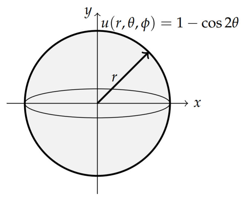
u(r,θ,ϕ)=1−cos2θ.
Solution
In problems in which there is no ϕ-dependence, only the m=0 terms of the general solution survives. Thus, we have that
u(ρ,θ,ϕ)=∞∑ℓ=0aℓρℓPℓ(cosθ).
Here we have used the fact that P0ℓ(x)=Pℓ(x). We just need to determine the unknown expansion coefficients, aℓ. Imposing the boundary condition at ρ=r, we are lead to
g(θ)=∞∑ℓ=0aℓrℓPℓ(cosθ)
This is a Fourier-Legendre series representation of g(θ). Since the Legendre polynomials are an orthogonal set of eigenfunctions, we can extract the coefficients.
In Chapter 5 we had proven that
∫π0Pn(cosθ)Pm(cosθ)sinθdθ=∫1−1Pn(x)Pm(x)dx=22n+1δnm.
So, multiplying the expression for g(θ) by Pm(cosθ)sinθ and integrating, we obtain the expansion coefficients:
aℓ=2ℓ+12rℓ∫π0g(θ)Pℓ(cosθ)sinθdθ.
Sometimes it is easier to rewrite g(θ) as a polynomial in cosθ and avoid the integration. For this example we see that
g(θ)=1−cos2θ=2sin2θ=2−2cos2θ.
Thus, setting x=cosθ and G(x)=g(θ(x)), we have G(x)=2−2x2.
We seek the form
G(x)=c0P0(x)+c1P1(x)+c2P2(x),
where P0(x)=1,P1(x)=x, and P2(x)=12(3x2−1). Since G(x)=2−2x2 does not have any x terms, we know that c1=0. So,
2−2x2=c0(1)+c212(3x2−1)=c0−12c2+32c2x2.
By observation we have c2=−43 and thus, c0=2+12c2=43. Therefore, G(x)=43P0(x)−43P2(x).
We have found the expansion of g(θ) in terms of Legendre polynomials,
g(θ)=43P0(cosθ)−43P2(cosθ).
Therefore, the nonzero coefficients in the general solution become
a0=43,a2=431r2,
and the rest of the coefficients are zero. Inserting these into the general solution, we have the final solution
u(ρ,θ,ϕ)=43P0(cosθ)−43(ρr)2P2(cosθ)=43−23(ρr)2(3cos2θ−1)
Spherical Harmonics
The solutions of the angular parts of the problem are often combined into one function of two variables, as problems with spherical symmetry arise often, leaving the main differences between such problems confined to the radial equation. These functions are referred to as spherical harmonics, Yℓm(θ,ϕ), which are defined with a special normalization as
Yℓm(θ,ϕ)=(−1)m√2ℓ+14π(ℓ−m)!(ℓ+m)!Pmℓ(cosθ)eimϕ.
These satisfy the simple orthogonality relation
∫π0∫2π0Yℓm(θ,ϕ)Y∗ℓ′m′(θ,ϕ)sinθdϕdθ=δℓℓ′δmm′.
Yℓm(θ,ϕ), are the spherical harmonics. Spherical harmonics are important in applications from atomic electron configurations to gravitational fields, planetary magnetic fields, and the cosmic microwave background radiation.
As seen earlier in the chapter, the spherical harmonics are eigenfunctions of the eigenvalue problem LY=−λY, where
L=1sinθ∂∂θ(sinθ∂∂θ)+1sin2θ∂2∂ϕ2.
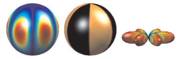
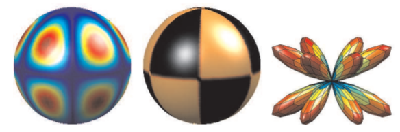
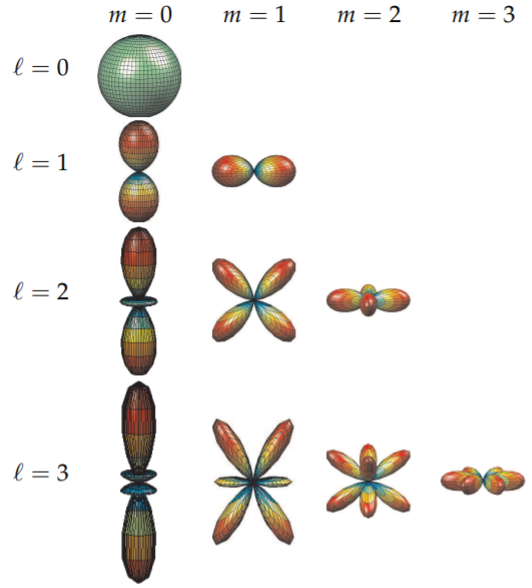
This operator appears in many problems in which there is spherical symmetry, such as obtaining the solution of Schrödinger’s equation for the hydrogen atom as we will see later. Therefore, it is customary to plot spherical harmonics. Because the Yℓm ’s are complex functions, one typically plots either the real part or the modulus squared. One rendition of |Yℓm(θ,ϕ)|2 is shown in Table 6.5.2 for ℓ,m=0,1,2,3.
Table 6.5.2: The first few spherical harmonics, |Yℓm(θ,ϕ)|2
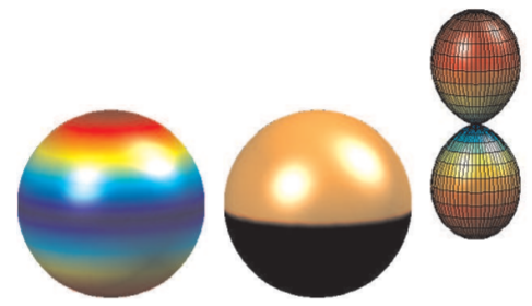
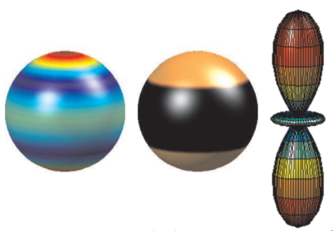
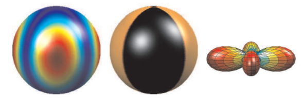
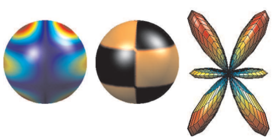
We could also look for the nodal curves of the spherical harmonics like we had for vibrating membranes. Such surface plots on a sphere are shown in Table 6.5.3. The colors provide for the amplitude of the |Yℓm(θ,φ)|2. We can match these with the shapes in Table 6.5.2 by coloring the plots with some of the same colors as shown in Table 6.5.3. However, by plotting just the sign of the spherical harmonics, as in Table 6.5.4, we can pick out the nodal curves much easier.
Table 6.5.3: Spherical harmonic contours for |Yℓm(θ,ϕ)|2.
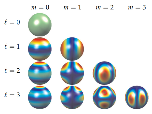
Table 6.5.4: In these figures we show the nodal curves of |Yℓm(θ,ϕ)|2 Along the first column (m=0) are the zonal harmonics seen as ℓ horizontal circles. Along the top diagonal (m=ℓ) are the sectional harmonics. These look like orange sections formed from m vertical circles. The remaining harmonics are tesseral harmonics. They look like a checkerboard pattern formed from intersections of ℓ−m horizontal circles and m vertical circles.
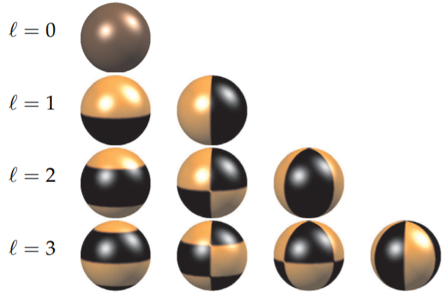
Spherical, or surface, harmonics can be further grouped into zonal, sectoral, and tesseral harmonics. Zonal harmonics correspond to the m=0 modes. In this case, one seeks nodal curves for which Pℓ(cosθ)=0. Solutions of this equation lead to constant θ values such that cosθ is a zero of the Legendre polynomial, Pℓ(x). The zonal harmonics correspond to the first column in Table 6.5.4. Since Pℓ(x) is a polynomial of degree ℓ, the zonal harmonics consist of ℓ latitudinal circles.
Sectoral, or meridional, harmonics result for the case that m=±ℓ. For this case, we note that P±ℓℓ(x)∝(1−x2)m/2. This function vanishes for x=±1, or θ=0,π. Therefore, the spherical harmonics can only produce nodal curves for eimϕ=0. Thus, one obtains the meridians satisfying the condition Acosmϕ+Bsinmϕ=0. Solutions of this equation are of the form ϕ= constant. These modes can be seen in Table 6.5.4 in the top diagonal and can be described as m circles passing through the poles, or longitudinal circles.
Tesseral harmonics consist of the rest of the modes, which typically look like a checker board glued to the surface of a sphere. Examples can be seen in the pictures of nodal curves, such as Table 6.5.4. Looking in Table 6.5.4 along the diagonals going downward from left to right, one can see the same number of latitudinal circles. In fact, there are ℓ−m latitudinal nodal curves in these figures.
In summary, the spherical harmonics have several representations, as show in Tables 6.5.3-6.5.4. Note that there are ℓ nodal lines, m meridional curves, and ℓ−m horizontal curves in these figures. The plots in Table 6.5.2 are the typical plots shown in physics for discussion of the wavefunctions of the hydrogen atom. Those in 6.5.3 are useful for describing gravitational or electric potential functions, temperature distributions, or wave modes on a spherical surface. The relationships between these pictures and the nodal curves can be better understood by comparing respective plots. Several modes were separated out in Figures 6.5.4-6.5.9 to make this comparison easier.