6.4: Three Dimensional Cake Baking

In the rest of the chapter we will extend our studies to three dimensional problems. In this section we will solve the heat equation as we look at examples of baking cakes.

We consider cake batter, which is at room temperature of $T_{i}=80^{\circ} \mathrm{F}$. It is placed into an oven, also at a fixed temperature, $T_{b}=350^{\circ} \mathrm{F}$. For simplicity, we will assume that the thermal conductivity and cake density are constant. Of course, this is not quite true. However, it is an approximation which simplifies the model. We will consider two cases, one in which the cake is a rectangular solid, such as baking it in a $13^{\prime \prime} \times 9^{\prime \prime} \times 2^{\prime \prime}$ baking pan. The other case will lead to a cylindrical cake, such as you would obtain from a round cake pan.

Note

This discussion of cake baking is adapted from R. Wilkinson’s thesis work. That in turn was inspired by work done by Dr. Olszewski,(2006) From baking a cake to solving the diffusion equation. American Journal of Physics $74(6)$.

Assuming that the heat constant $k$ is indeed constant and the temperature is given by $T(\mathbf{r}, t)$, we begin with the heat equation in three dimensions,

$$\frac{\partial T}{\partial t}=k \nabla^{2} T \text {. }\label{eq:1}$$

We will need to specify initial and boundary conditions. Let $T_{i}$ be the initial batter temperature, $T(x, y, z, 0)=T_{i}$.

We choose the boundary conditions to be fixed at the oven temperature $T_{b}$. However, these boundary conditions are not homogeneous and would lead to problems when carrying out separation of variables. This is easily remedied by subtracting the oven temperature from all temperatures involved and defining $u(\mathbf{r}, t)=T(\mathbf{r}, t)-T_{b}$. The heat equation then becomes

$$\frac{\partial u}{\partial t}=k \nabla^{2} u\label{eq:2}$$

with initial condition

$$u(\mathbf{r}, 0)=T_{i}-T_{b} .\nonumber$$

The boundary conditions are now homogeneous. We cannot be any more specific than this until we specify the geometry.

Example $\PageIndex{1}$: Temperature of a Rectangular Cake

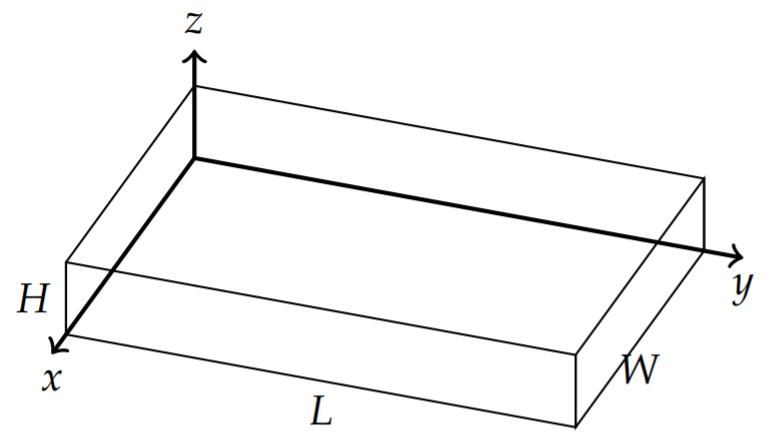
We will consider a rectangular cake with dimensions $0 \leq x \leq W, 0 \leq y \leq L$, and $0 \leq z \leq H$ as show in Figure $\PageIndex{1}$. For this problem, we seek solutions of the heat equation plus the conditions

$$\begin{aligned} u(x, y, z, 0) &=T_{i}-T_{b}, \\ u(0, y, z, t)=u(W, y, z, t) &=0, \\ u(x, 0, z, t)=u(x, L, z, t) &=0, \\ u(x, y, 0, t)=u(x, y, H, t) &=0 . \end{aligned} \nonumber$$

Figure $\PageIndex{1}$: The dimensions of a rectangular cake.

Solution

Using the method of separation of variables, we seek solutions of the form

$$u(x, y, z, t)=X(x) Y(y) Z(z) G(t) .\label{eq:3}$$

Substituting this form into the heat equation, we get

$$\frac{1}{k} \frac{G^{\prime}}{G}=\frac{X^{\prime \prime}}{X}+\frac{Y^{\prime \prime}}{Y}+\frac{Z^{\prime \prime}}{Z} .\label{eq:4}$$

Setting these expressions equal to $-\lambda$, we get

$$\frac{1}{k} \frac{G^{\prime}}{G}=-\lambda \quad \text { and } \quad \frac{X^{\prime \prime}}{X}+\frac{Y^{\prime \prime}}{Y}+\frac{Z^{\prime \prime}}{Z}=-\lambda\label{eq:5}$$

Therefore, the equation for $G(t)$ is given by

$$G^{\prime}+k \lambda G=0 .\nonumber$$

We further have to separate out the functions of $x, y$, and $z$. We anticipate that the homogeneous boundary conditions will lead to oscillatory solutions in these variables. Therefore, we expect separation of variables will lead to the eigenvalue problems

$$\begin{align} X^{\prime \prime}+\mu^{2} X &=0, & X(0) &=X(W)=0,\nonumber \\ Y^{\prime \prime}+v^{2} Y &=0, & Y(0) &=Y(L)=0,\nonumber \\ Z^{\prime \prime}+\kappa^{2} Z &=0, & Z(0) &=Z(H)=0 .\label{eq:6} \end{align}$$

Noting that

$$\frac{X^{\prime \prime}}{X}=-\mu^{2}, \quad \frac{Y^{\prime \prime}}{Y}=-v^{2}, \quad \frac{Z^{\prime \prime}}{Z}=-\kappa^{2},\nonumber$$

we find from the heat equation that the separation constants are related,

$$\lambda^{2}=\mu^{2}+v^{2}+\kappa^{2} .\nonumber$$

We could have gotten to this point quicker by writing the first separated equation labeled with the separation constants as

$$\underbrace{\frac{1}{k} \frac{G^{\prime}}{G}}_{-\lambda}=\underbrace{\frac{X^{\prime \prime}}{X}}_{-\mu}+\underbrace{\frac{Y^{\prime \prime}}{Y}}_{-v}+\underbrace{\frac{Z^{\prime \prime}}{Z}}_{-\kappa} .\nonumber$$

Then, we can read off the eigenvalues problems and determine that $\lambda^{2}=\mu^{2}+v^{2}+$ $\kappa^{2}$.

From the boundary conditions, we get product solutions for $u(x, y, z, t)$ in the form

$$u_{m n \ell}(x, y, z, t)=\sin \mu_{m} x \sin v_{n} y \sin \kappa_{\ell} z e^{-\lambda_{m n} k t},\nonumber$$

for

$$\lambda_{m n l}=\mu_{m}^{2}+v_{n}^{2}+\kappa_{\ell}^{2}=\left(\frac{m \pi}{W}\right)^{2}+\left(\frac{n \pi}{L}\right)^{2}+\left(\frac{\ell \pi}{H}\right)^{2}, \quad m, n, \ell=1,2, \ldots\nonumber$$

The general solution is a linear combination of all of the product solutions, summed over three different indices,

$$u(x, y, z, t)=\sum_{m=1}^{\infty} \sum_{n=1}^{\infty} \sum_{\ell=1}^{\infty} A_{m n l} \sin \mu_{m} x \sin v_{n} y \sin \kappa_{\ell} z e^{-\lambda_{m n} k t},\label{eq:7}$$

where the $A_{\text {mn }}$ ’s are arbitrary constants.

Figure $\PageIndex{2}$: Rectangular cake showing a vertical slice.

We can use the initial condition $u(x,y,z,0)=T_i-T_b$ to determine the $A_{mn\ell}$'s. We find

$$\label{eq:8}T_i-T_b=\sum\limits_{m=1}^\infty\sum\limits_{n=1}^\infty\sum\limits_{\ell =1}^\infty A_{mnl}\sin\mu_m x\sin v_ny\sin k_{\ell} z.$$

This is a triple Fourier sine series.

We can determine these coefficients in a manner similar to how we handled double Fourier sine series earlier in the chapter. Defining

$$b_m(y,z)=\sum\limits_{n=1}^\infty\sum\limits_{\ell =1}^\infty A_{mnl}\sin v_ny\sin k_{\ell}z,\nonumber$$

we obtain a simple Fourier sine series:

$$T_i-T_b=\sum\limits_{m=1}^\infty b_m(y,z)\sin\mu_mx.\label{eq:9}$$

The Fourier coefficients can then be found as

$$b_m(y,z)=\frac{2}{W}\int_0^W (T_i-T_b)\sin\mu_mxdx.\nonumber$$

Using the same technique for the remaining sine series and noting that $T_i − T_b$ is constant, we can determine the general coefficients $A_{mnl}$ by carrying out the needed integrations:

$$\begin{aligned}A_{mnl}&=\frac{8}{WLH}\int_0^H\int_0^L\int_0^W (T_i-T_b)\sin\mu_m x\sin v_ny\sin k_{\ell}zdxdydz \\ &=(T_i-T_b)\frac{8}{\pi^3}\left[\frac{\cos\left(\frac{m\pi x}{W}\right)}{m}\right]_0^W \left[\frac{\cos\left(\frac{n\pi y}{L}\right)}{n}\right]_0^L \left[\frac{\cos\left(\frac{\ell\pi z}{H}\right)}{\ell}\right]_0^H \\ &=(T_i-T_b)\frac{8}{\pi^3}\left[\frac{\cos m\pi -1}{m}\right]\left[\frac{\cos n\pi -1}{n}\right]\left[\frac{\cos\ell\pi -1}{\ell}\right] \\ &=(T_i-T_b)\frac{8}{\pi^3}\left\{\begin{array}{ll} 0,&\text{for at least one }m,n,\ell\text{ even,} \\ \left[\frac{-2}{m}\right]\left[\frac{-2}{n}\right]\left[\frac{-2}{\ell}\right],&\text{for }m,n,\ell\text{ all odd.}\end{array}\right.\end{aligned} \nonumber$$

Since only the odd multiples yield non-zero $A_{mn\ell}$ we let $m=2m'-1$, $n=2n'-1$, and $\ell =2\ell '-1$ for $m',n',\ell '=1,2,\ldots$. The expansion coefficients can now be written in the simpler form

$$A_{mn}=\frac{64(T_b-T_i)}{(2m'-1)(2n'-1)(2\ell '-1)\pi ^3}.\nonumber$$

Substituting this result into general solution and dropping the primes, we find

$$u(x,y,z,t)=\frac{64(T_b-T_i)}{\pi^3}\sum\limits_{m=1}^\infty\sum\limits_{n=1}^\infty\sum\limits_{\ell =1}^\infty \frac{\sin\mu_m x\sin v_ny\sin k_{\ell}ze^{-\lambda_{mnt}kt}}{(2m-1)(2n-1)(2\ell -1)},\nonumber$$

where

$$\lambda_{m n \ell}=\left(\frac{(2 m-1) \pi}{W}\right)^{2}+\left(\frac{(2 n-1) \pi}{L}\right)^{2}+\left(\frac{(2 \ell-1) \pi}{H}\right)^{2}\nonumber$$

for $m, n, \ell=1,2, \ldots . .$

Recalling that the solution to the physical problem is

$$T(x, y, z, t)=u(x, y, z, t)+T_{b},\nonumber$$

we have the final solution is given by

$$T(x, y, z, t)=T_{b}+\frac{64\left(T_{b}-T_{i}\right)}{\pi^{3}} \sum_{m=1}^{\infty} \sum_{n=1}^{\infty} \sum_{\ell=1}^{\infty} \frac{\sin \hat{\mu}_{m} x \sin \hat{v}_{n} y \sin \hat{\kappa}_{\ell} z e^{-\hat{\lambda}_{m n \ell} k t}}{(2 m-1)(2 n-1)(2 \ell-1)}\nonumber$$

Figure $\PageIndex{3}$: Temperature evolution for a $13^{\prime \prime} \times 9^{\prime \prime} \times 2^{\prime \prime}$ cake shown as vertical slices at the indicated length in feet.

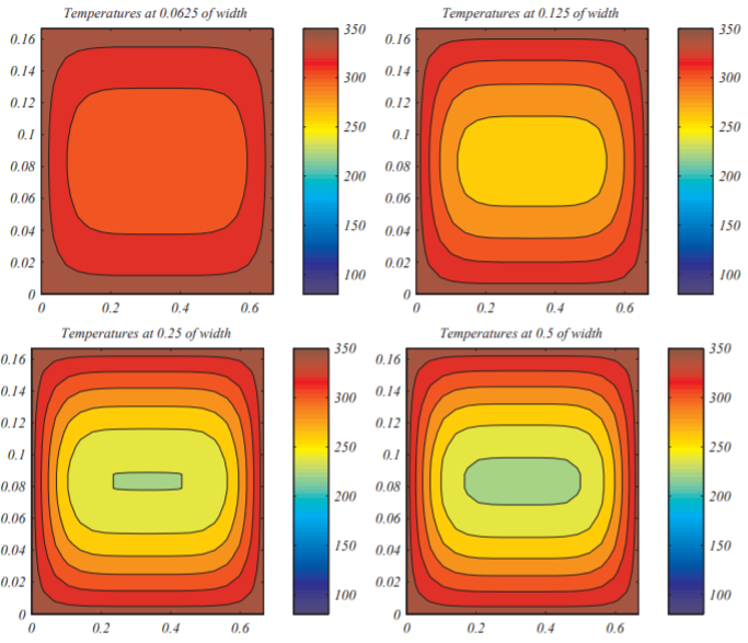
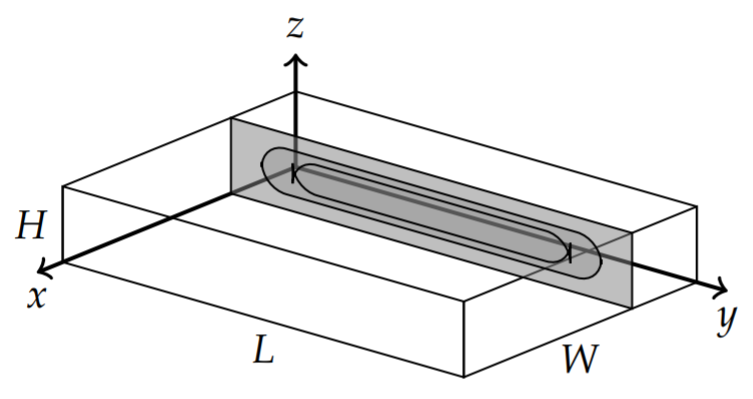
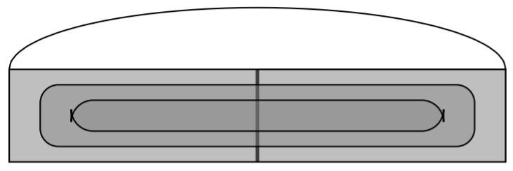
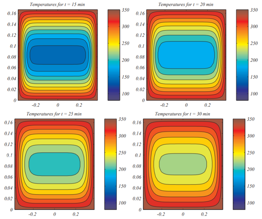
We show some temperature distributions in Figure $\PageIndex{3}$. Since we cannot capture the entire cake, we show vertical slices such as depicted in Figure $\PageIndex{2}$. Vertical slices are taken at the positions and times indicated for a $13^{\prime \prime} \times 9^{\prime \prime} \times 2^{\prime \prime}$ cake. Obviously, this is not accurate because the cake consistency is changing and this will affect the parameter $k$. A more realistic model would be to allow $k = k(T(x, y, z, t))$. However, such problems are beyond the simple methods described in this book.

Example $\PageIndex{2}$: Circular Cakes

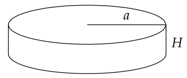
In this case the geometry of the cake is cylindrical as show in Figure $\PageIndex{4}$. Therefore, we need to express the boundary conditions and heat equation in cylindrical coordinates. Also, we will assume that the solution, $u(r, z, t)=T(r, z, t)-T_{b}$, is independent of $\theta$ due to axial symmetry. This gives the heat equation in $\theta$ independent cylindrical coordinates as

$$\frac{\partial u}{\partial t}=k\left(\frac{1}{r} \frac{\partial}{\partial r}\left(r \frac{\partial u}{\partial r}\right)+\frac{\partial^{2} u}{\partial z^{2}}\right),\label{eq:10}$$

where $0 \leq r \leq a$ and $0 \leq z \leq Z$. The initial condition is

$$u(r, z, 0)=T_{i}-T_{b},\nonumber$$

and the homogeneous boundary conditions on the side, top, and bottom of the cake are

$$\begin{array}{r} u(a, z, t)=0, \\ u(r, 0, t)=u(r, Z, t)=0 . \end{array}\nonumber$$

Figure $\PageIndex{4}$: Geometry for a cylindrical cake.

Solution

Again, we seek solutions of the form $u(r, z, t)=R(r) H(z) G(t)$. Separation of variables leads to

$$\underbrace{\frac{1}{k} \frac{G^{\prime}}{G}}_{-\lambda}=\underbrace{\frac{1}{r R} \frac{d}{d r}\left(r R^{\prime}\right)}_{-\mu^{2}}+\underbrace{\frac{H^{\prime \prime}}{H}}_{-v^{2}} .\label{eq:11}$$

Here we have indicated the separation constants, which lead to three ordinary differential equations. These equations and the boundary conditions are

$$\begin{align} G^{\prime}+k \lambda G &=0,\nonumber \\ \frac{d}{d r}\left(r R^{\prime}\right)+\mu^{2} r R &=0, \quad R(a)=0, \quad R(0) \text { is finite, }\nonumber \\ H^{\prime \prime}+v^{2} H &=0, \quad H(0)=H(Z)=0 .\label{eq:12} \end{align}$$

We further note that the separation constants are related by $\lambda=\mu^{2}+v^{2}$.

We can easily write down the solutions for $G(t)$ and $H(z)$,

$$G(t)=A e^{-\lambda k t}\nonumber$$

and

$$H_{n}(z)=\sin \frac{n \pi z}{Z}, \quad n=1,2,3, \ldots,\nonumber$$

where $v=\frac{n \pi}{Z}$. Recalling from the rectangular case that only odd terms arise in the Fourier sine series coefficients for the constant initial condition, we proceed by rewriting $H(z)$ as

$$H_{n}(z)=\sin \frac{(2 n-1) \pi z}{Z}, \quad n=1,2,3, \ldots\label{eq:13}$$

with $v=\frac{(2 n-1) \pi}{Z}$.

The radial equation can be written in the form

$$r^{2} R^{\prime \prime}+r R^{\prime}+\mu^{2} r^{2} R=0 .\nonumber$$

This is a Bessel equation of the first kind of order zero which we had seen in Section 5.5. Therefore, the general solution is a linear combination of Bessel functions of the first and second kind,

$$R(r)=c_{1} J_{0}(\mu r)+c_{2} N_{0}(\mu r) .\label{eq:14}$$

Since $R(r)$ is bounded at $r=0$ and $N_{0}(\mu r)$ is not well behaved at $r=0$, we set $c_{2}=0$. Up to a constant factor, the solution becomes

$$R(r)=J_{0}(\mu r) .\label{eq:15}$$

The boundary condition $R(a)=0$ gives the eigenvalues as

$$\mu_{m}=\frac{j_{0 m}}{a}, \quad m=1,2,3, \ldots,\nonumber$$

where $j_{0 m}$ is the $m^{\text {th }}$ roots of the zeroth-order Bessel function, $J_{0}\left(j_{0 m}\right)=0$.

Therefore, we have found the product solutions

$$H_{n}(z) R_{m}(r) G(t)=\sin \frac{(2 n-1) \pi z}{\mathrm{Z}} J_{0}\left(\frac{r}{a} j_{0 m}\right) e^{-\lambda_{n m} k t},\label{eq:16}$$

where $m=1,2,3, \ldots, n=1,2, \ldots$. Combining the product solutions, the general solution is found as

$$u(r, z, t)=\sum_{n=1}^{\infty} \sum_{m=1}^{\infty} A_{n m} \sin \frac{(2 n-1) \pi z}{Z} J_{0}\left(\frac{r}{a} j_{0 m}\right) e^{-\lambda_{n m} k t}\label{eq:17}$$

with

$$\lambda_{n m}=\left(\frac{(2 n-1) \pi}{\mathrm{Z}}\right)^{2}+\left(\frac{j_{0 m}}{a}\right)^{2},\nonumber$$

for $n, m=1,2,3, \ldots$.

Inserting the solution into the constant initial condition, we have

$$T_{i}-T_{b}=\sum_{n=1}^{\infty} \sum_{m=1}^{\infty} A_{n m} \sin \frac{(2 n-1) \pi z}{\mathrm{Z}} J_{0}\left(\frac{r}{a} j_{0 m}\right) .\nonumber$$

This is a double Fourier series but it involves a Fourier-Bessel expansion. Writing

$$b_{n}(r)=\sum_{m=1}^{\infty} A_{n m} J_{0}\left(\frac{r}{a} j_{0 m}\right),\nonumber$$

the condition becomes

$$T_{i}-T_{b}=\sum_{n=1}^{\infty} b_{n}(r) \sin \frac{(2 n-1) \pi z}{Z} .\nonumber$$

As seen previously, this is a Fourier sine series and the Fourier coefficients are given by

$$\begin{aligned} b_{n}(r) &=\frac{2}{Z} \int_{0}^{Z}\left(T_{i}-T_{b}\right) \sin \frac{(2 n-1) \pi z}{Z} d z \\ &=\frac{2\left(T_{i}-T_{b}\right)}{Z}\left[-\frac{Z}{(2 n-1) \pi} \cos \frac{(2 n-1) \pi z}{Z}\right]_{0}^{Z} \\ &=\frac{4\left(T_{i}-T_{b}\right)}{(2 n-1) \pi} \end{aligned} \nonumber$$

We insert this result into the Fourier-Bessel series,

$$\frac{4\left(T_{i}-T_{b}\right)}{(2 n-1) \pi}=\sum_{m=1}^{\infty} A_{n m} J_{0}\left(\frac{r}{a} j_{0 m}\right),\nonumber$$

and recall from Section 5.5 that we can determine the Fourier coefficients $A_{n m}$ using the Fourier-Bessel series,

$$f(x)=\sum_{n=1}^{\infty} c_{n} J_{p}\left(j_{p n} \frac{x}{a}\right),\label{eq:18}$$

where the Fourier-Bessel coefficients are found as

$$c_{n}=\frac{2}{a^{2}\left[J_{p+1}\left(j_{p n}\right)\right]^{2}} \int_{0}^{a} x f(x) J_{p}\left(j_{p n} \frac{x}{a}\right) d x .\label{eq:19}$$

Comparing these series expansions, we have

$$A_{n m}=\frac{2}{a^{2} J_{1}^{2}\left(j_{0 m}\right)} \frac{4\left(T_{i}-T_{b}\right)}{(2 n-1) \pi} \int_{0}^{a} J_{0}\left(\mu_{m} r\right) r d r .\label{eq:20}$$

In order to evaluate $\int_{0}^{a} J_{0}\left(\mu_{m} r\right) r d r$, we let $y=\mu_{m} r$ and get

$$\begin{align} \int_{0}^{a} J_{0}\left(\mu_{m} r\right) r d r &=\int_{0}^{\mu_{m} a} J_{0}(y) \frac{y}{\mu_{m}} \frac{d y}{\mu_{m}}\nonumber \\ &=\frac{1}{\mu_{m}^{2}} \int_{0}^{\mu_{m} a} J_{0}(y) y d y\nonumber \\ &=\frac{1}{\mu_{m}^{2}} \int_{0}^{\mu_{m} a} \frac{d}{d y}\left(y J_{1}(y)\right) d y\nonumber \\ &=\frac{1}{\mu_{m}^{2}}\left(\mu_{m} a\right) J_{1}\left(\mu_{m} a\right)=\frac{a^{2}}{j_{0 m}} J_{1}\left(j_{0 m}\right) .\label{eq:21} \end{align}$$

Here we have made use of the identity $\frac{d}{d x}\left(x J_{1}(x)\right)=J_{0}(x)$ from Section 5.5.

Substituting the result of this integral computation into the expression for $A_{n m}$, we find

$$A_{n m}=\frac{8\left(T_{i}-T_{b}\right)}{(2 n-1) \pi} \frac{1}{j_{0 m} J_{1}\left(j_{0 m}\right)} .\nonumber$$

Substituting this result into the original expression for $u(r, z, t)$, gives

$$u(r, z, t)=\frac{8\left(T_{i}-T_{b}\right)}{\pi} \sum_{n=1}^{\infty} \sum_{m=1}^{\infty} \frac{\sin \frac{(2 n-1) \pi z}{Z}}{(2 n-1)} \frac{J_{0}\left(\frac{r}{a} j 0 m\right) e^{-\lambda_{m m} k t}}{j_{0 m} J_{1}\left(j_{0 m}\right)} .\nonumber$$

Therefore, $T(r, z, t)$ is found as

$$T(r, z, t)=T_{b}+\frac{8\left(T_{i}-T_{b}\right)}{\pi} \sum_{n=1}^{\infty} \sum_{m=1}^{\infty} \frac{\sin \frac{(2 n-1) \pi z}{Z}}{(2 n-1)} \frac{J_{0}\left(\frac{r}{a} j_{0 m}\right) e^{-\lambda_{n m} k t}}{j_{0 m} J_{1}\left(j_{0 m}\right)},\nonumber$$

where

$$\lambda_{n m}=\left(\frac{(2 n-1) \pi}{\mathrm{Z}}\right)^{2}+\left(\frac{j_{0 m}}{a}\right)^{2}, \quad n, m=1,2,3, \ldots .\nonumber$$

We have therefore found the general solution for the three-dimensional heat equation in cylindrical coordinates with constant diffusivity. Similar to the solutions shown in Figure $\PageIndex{3}$ of the previous section, we show in Figure $\PageIndex{6}$ the temperature evolution throughout a standard $9^{\prime \prime}$ round cake pan. These are vertical slices similar to what is depicted in Figure $\PageIndex{5}$.

Figure $\PageIndex{5}$: Depiction of a sideview of a vertical slice of a circular cake.

Figure $\PageIndex{6}$: Temperature evolution for a standard $9''$ cake shown as vertical slices through the center.

Again, one could generalize this example to considerations of other types of cakes with cylindrical symmetry. For example, there are muffins, Boston steamed bread which is steamed in tall cylindrical cans. One could also consider an annular pan, such as a bundt cake pan. In fact, such problems extend beyond baking cakes to possible heating molds in manufacturing.