
6.2: Vibrations of a Kettle Drum
- Page ID
- 90265

\( \newcommand{\vecs}[1]{\overset { \scriptstyle \rightharpoonup} {\mathbf{#1}} } \)
\( \newcommand{\vecd}[1]{\overset{-\!-\!\rightharpoonup}{\vphantom{a}\smash {#1}}} \)
\( \newcommand{\dsum}{\displaystyle\sum\limits} \)
\( \newcommand{\dint}{\displaystyle\int\limits} \)
\( \newcommand{\dlim}{\displaystyle\lim\limits} \)
\( \newcommand{\id}{\mathrm{id}}\) \( \newcommand{\Span}{\mathrm{span}}\)
( \newcommand{\kernel}{\mathrm{null}\,}\) \( \newcommand{\range}{\mathrm{range}\,}\)
\( \newcommand{\RealPart}{\mathrm{Re}}\) \( \newcommand{\ImaginaryPart}{\mathrm{Im}}\)
\( \newcommand{\Argument}{\mathrm{Arg}}\) \( \newcommand{\norm}[1]{\| #1 \|}\)
\( \newcommand{\inner}[2]{\langle #1, #2 \rangle}\)
\( \newcommand{\Span}{\mathrm{span}}\)
\( \newcommand{\id}{\mathrm{id}}\)
\( \newcommand{\Span}{\mathrm{span}}\)
\( \newcommand{\kernel}{\mathrm{null}\,}\)
\( \newcommand{\range}{\mathrm{range}\,}\)
\( \newcommand{\RealPart}{\mathrm{Re}}\)
\( \newcommand{\ImaginaryPart}{\mathrm{Im}}\)
\( \newcommand{\Argument}{\mathrm{Arg}}\)
\( \newcommand{\norm}[1]{\| #1 \|}\)
\( \newcommand{\inner}[2]{\langle #1, #2 \rangle}\)
\( \newcommand{\Span}{\mathrm{span}}\) \( \newcommand{\AA}{\unicode[.8,0]{x212B}}\)
\( \newcommand{\vectorA}[1]{\vec{#1}} % arrow\)
\( \newcommand{\vectorAt}[1]{\vec{\text{#1}}} % arrow\)
\( \newcommand{\vectorB}[1]{\overset { \scriptstyle \rightharpoonup} {\mathbf{#1}} } \)
\( \newcommand{\vectorC}[1]{\textbf{#1}} \)
\( \newcommand{\vectorD}[1]{\overrightarrow{#1}} \)
\( \newcommand{\vectorDt}[1]{\overrightarrow{\text{#1}}} \)
\( \newcommand{\vectE}[1]{\overset{-\!-\!\rightharpoonup}{\vphantom{a}\smash{\mathbf {#1}}}} \)
\( \newcommand{\vecs}[1]{\overset { \scriptstyle \rightharpoonup} {\mathbf{#1}} } \)
\(\newcommand{\longvect}{\overrightarrow}\)
\( \newcommand{\vecd}[1]{\overset{-\!-\!\rightharpoonup}{\vphantom{a}\smash {#1}}} \)
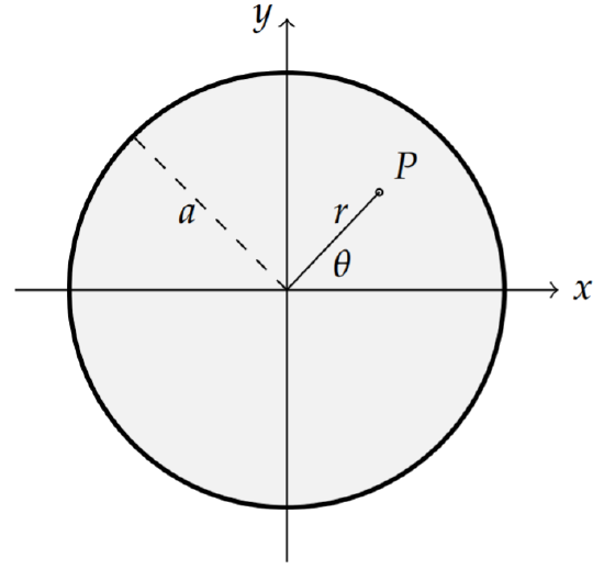
\(\newcommand{\avec}{\mathbf a}\) \(\newcommand{\bvec}{\mathbf b}\) \(\newcommand{\cvec}{\mathbf c}\) \(\newcommand{\dvec}{\mathbf d}\) \(\newcommand{\dtil}{\widetilde{\mathbf d}}\) \(\newcommand{\evec}{\mathbf e}\) \(\newcommand{\fvec}{\mathbf f}\) \(\newcommand{\nvec}{\mathbf n}\) \(\newcommand{\pvec}{\mathbf p}\) \(\newcommand{\qvec}{\mathbf q}\) \(\newcommand{\svec}{\mathbf s}\) \(\newcommand{\tvec}{\mathbf t}\) \(\newcommand{\uvec}{\mathbf u}\) \(\newcommand{\vvec}{\mathbf v}\) \(\newcommand{\wvec}{\mathbf w}\) \(\newcommand{\xvec}{\mathbf x}\) \(\newcommand{\yvec}{\mathbf y}\) \(\newcommand{\zvec}{\mathbf z}\) \(\newcommand{\rvec}{\mathbf r}\) \(\newcommand{\mvec}{\mathbf m}\) \(\newcommand{\zerovec}{\mathbf 0}\) \(\newcommand{\onevec}{\mathbf 1}\) \(\newcommand{\real}{\mathbb R}\) \(\newcommand{\twovec}[2]{\left[\begin{array}{r}#1 \\ #2 \end{array}\right]}\) \(\newcommand{\ctwovec}[2]{\left[\begin{array}{c}#1 \\ #2 \end{array}\right]}\) \(\newcommand{\threevec}[3]{\left[\begin{array}{r}#1 \\ #2 \\ #3 \end{array}\right]}\) \(\newcommand{\cthreevec}[3]{\left[\begin{array}{c}#1 \\ #2 \\ #3 \end{array}\right]}\) \(\newcommand{\fourvec}[4]{\left[\begin{array}{r}#1 \\ #2 \\ #3 \\ #4 \end{array}\right]}\) \(\newcommand{\cfourvec}[4]{\left[\begin{array}{c}#1 \\ #2 \\ #3 \\ #4 \end{array}\right]}\) \(\newcommand{\fivevec}[5]{\left[\begin{array}{r}#1 \\ #2 \\ #3 \\ #4 \\ #5 \\ \end{array}\right]}\) \(\newcommand{\cfivevec}[5]{\left[\begin{array}{c}#1 \\ #2 \\ #3 \\ #4 \\ #5 \\ \end{array}\right]}\) \(\newcommand{\mattwo}[4]{\left[\begin{array}{rr}#1 \amp #2 \\ #3 \amp #4 \\ \end{array}\right]}\) \(\newcommand{\laspan}[1]{\text{Span}\{#1\}}\) \(\newcommand{\bcal}{\cal B}\) \(\newcommand{\ccal}{\cal C}\) \(\newcommand{\scal}{\cal S}\) \(\newcommand{\wcal}{\cal W}\) \(\newcommand{\ecal}{\cal E}\) \(\newcommand{\coords}[2]{\left\{#1\right\}_{#2}}\) \(\newcommand{\gray}[1]{\color{gray}{#1}}\) \(\newcommand{\lgray}[1]{\color{lightgray}{#1}}\) \(\newcommand{\rank}{\operatorname{rank}}\) \(\newcommand{\row}{\text{Row}}\) \(\newcommand{\col}{\text{Col}}\) \(\renewcommand{\row}{\text{Row}}\) \(\newcommand{\nul}{\text{Nul}}\) \(\newcommand{\var}{\text{Var}}\) \(\newcommand{\corr}{\text{corr}}\) \(\newcommand{\len}[1]{\left|#1\right|}\) \(\newcommand{\bbar}{\overline{\bvec}}\) \(\newcommand{\bhat}{\widehat{\bvec}}\) \(\newcommand{\bperp}{\bvec^\perp}\) \(\newcommand{\xhat}{\widehat{\xvec}}\) \(\newcommand{\vhat}{\widehat{\vvec}}\) \(\newcommand{\uhat}{\widehat{\uvec}}\) \(\newcommand{\what}{\widehat{\wvec}}\) \(\newcommand{\Sighat}{\widehat{\Sigma}}\) \(\newcommand{\lt}{<}\) \(\newcommand{\gt}{>}\) \(\newcommand{\amp}{&}\) \(\definecolor{fillinmathshade}{gray}{0.9}\)In this section we consider the vibrations of a circular membrane of radius \(a\) as shown in Figure \(\PageIndex{1}\). Again we are looking for the harmonics of the vibrating membrane, but with the membrane fixed around the circular boundary given by \(x^{2}+y^{2}=a^{2}\). However, expressing the boundary condition in Cartesian coordinates is awkward. Namely, we can only write \(u(x, y, t)=0\) for \(x^{2}+y^{2}=a^{2}\). It is more natural to use polar coordinates as indicated in Figure \(\PageIndex{1}\). Let the height of the membrane be given by \(u=u(r, \theta, t)\) at time \(t\) and position \((r, \theta)\). Now the boundary condition is given as \(u(a, \theta, t)=0\) for all \(t>0\) and \(\theta \in[0,2 \pi]\).
Before solving the initial-boundary value problem, we have to cast the full problem in polar coordinates. This means that we need to rewrite the Laplacian in \(r\) and \(\theta\). To do so would require that we know how to transform derivatives in \(x\) and \(y\) into derivatives with respect to \(r\) and \(\theta\). Using the results from Section ?? on curvilinear coordinates, we know that the Laplacian can be written in polar coordinates. In fact, we could use the results from Problem ?? in Chapter ?? for cylindrical coordinates for functions which are \(z\)-independent, \(f=f(r, \theta)\). Then, we would have
\[\nabla^{2} f=\frac{1}{r} \frac{\partial}{\partial r}\left(r \frac{\partial f}{\partial r}\right)+\frac{1}{r^{2}} \frac{\partial^{2} f}{\partial \theta^{2}} .\nonumber \]
We can obtain this result using a more direct approach, namely applying the Chain Rule in higher dimensions. First recall the transformations between polar and Cartesian coordinates:
\[x=r \cos \theta, \quad y=r \sin \theta\nonumber \]
and
\[r=\sqrt{x^{2}+y^{2}}, \quad \tan \theta=\frac{y}{x} .\nonumber \]
Now, consider a function \(f=f(x(r, \theta), y(r, \theta))=g(r, \theta)\). (Technically, once we transform a given function of Cartesian coordinates we obtain a new function \(g\) of the polar coordinates. Many texts do not rigorously distinguish between the two functions.) Thinking of \(x=x(r, \theta)\) and \(y=y(r, \theta)\), we have from the chain rule for functions of two variables:
\[\begin{align} \frac{\partial f}{\partial x} &=\frac{\partial g}{\partial r} \frac{\partial r}{\partial x}+\frac{\partial g}{\partial \theta} \frac{\partial \theta}{\partial x}\nonumber \\ &=\frac{\partial g}{\partial r} \frac{x}{r}-\frac{\partial g}{\partial \theta} \frac{y}{r^{2}}\nonumber \\ &=\cos \theta \frac{\partial g}{\partial r}-\frac{\sin \theta \partial g}{r} \frac{\partial g}{\partial \theta} .\label{eq:1} \end{align} \]
Here we have used
\[\frac{\partial r}{\partial x}=\frac{x}{\sqrt{x^{2}+y^{2}}}=\frac{x}{r}\nonumber \]
and
\[\frac{\partial \theta}{\partial x}=\frac{d}{d x}\left(\tan ^{-1} \frac{y}{x}\right)=\frac{-y / x^{2}}{1+\left(\frac{y}{x}\right)^{2}}=-\frac{y}{r^{2}} .\nonumber \]
Similarly,
\[\begin{align} \frac{\partial f}{\partial y} &=\frac{\partial g}{\partial r} \frac{\partial r}{\partial y}+\frac{\partial g}{\partial \theta} \frac{\partial \theta}{\partial y}\nonumber \\ &=\frac{\partial g}{\partial r} \frac{y}{r}+\frac{\partial g}{\partial \theta} \frac{x}{r^{2}}\nonumber \\ &=\sin \theta \frac{\partial g}{\partial r}+\frac{\cos \theta}{r} \frac{\partial g}{\partial \theta} .\label{eq:2} \end{align} \]
The \(2 \mathrm{D}\) Laplacian can now be computed as
\[\begin{align} \frac{\partial^{2} f}{\partial x^{2}}+\frac{\partial^{2} f}{\partial y^{2}}=& \cos \theta \frac{\partial}{\partial r}\left(\frac{\partial f}{\partial x}\right)-\frac{\sin \theta}{r} \frac{\partial}{\partial \theta}\left(\frac{\partial f}{\partial x}\right)\nonumber \\ &+\sin \theta \frac{\partial}{\partial r}\left(\frac{\partial f}{\partial y}\right)+\frac{\cos \theta}{r} \frac{\partial}{\partial \theta}\left(\frac{\partial f}{\partial y}\right) \nonumber \\ =& \cos \theta \frac{\partial}{\partial r}\left(\cos \theta \frac{\partial g}{\partial r}-\frac{\sin \theta}{r} \frac{\partial g}{\partial \theta}\right)\nonumber \\ &-\frac{\sin \theta}{r} \frac{\partial}{\partial \theta}\left(\cos \theta \frac{\partial g}{\partial r}-\frac{\sin \theta}{r} \frac{\partial g}{\partial \theta}\right)\nonumber \\ &+\sin \theta \frac{\partial}{\partial r}\left(\sin \theta \frac{\partial g}{\partial r}+\frac{\cos \theta}{r} \frac{\partial g}{\partial \theta}\right)\nonumber \\ &+\frac{\cos \theta}{r} \frac{\partial}{\partial \theta}\left(\sin \theta \frac{\partial g}{\partial r}+\frac{\cos \theta}{r} \frac{\partial g}{\partial \theta}\right)\nonumber \\ =& \cos \theta\left(\cos \theta \frac{\partial^{2} g}{\partial r^{2}}+\frac{\sin \theta}{r^{2}} \frac{\partial g}{\partial \theta}-\frac{\sin \theta}{r} \frac{\partial^{2} g}{\partial r \partial \theta}\right)\nonumber \\ &-\frac{\sin \theta}{r}\left(\cos \theta \frac{\partial^{2} g}{\partial \theta \partial r}-\frac{\sin \theta}{r} \frac{\partial^{2} g}{\partial \theta^{2}}-\sin \theta \frac{\partial g}{\partial r}-\frac{\cos \theta}{r} \frac{\partial g}{\partial \theta}\right)\nonumber \\ &+\sin \theta\left(\sin \theta \frac{\partial^{2} g}{\partial r^{2}}+\frac{\cos \theta}{r} \frac{\partial^{2} g}{\partial r \partial \theta}-\frac{\cos \theta}{r^{2}} \frac{\partial g}{\partial \theta}\right)\nonumber \\ &+\frac{\cos \theta}{r}\left(\sin \theta \frac{\partial^{2} g}{\partial \theta \partial r}+\frac{\cos \theta}{r} \frac{\partial^{2} g}{\partial \theta^{2}}+\cos \theta \frac{\partial g}{\partial r}-\frac{\sin \theta}{r} \frac{\partial g}{\partial \theta}\right)\nonumber \\ =& \frac{\partial^{2} g}{\partial r^{2}}+\frac{1}{r} \frac{\partial g}{\partial r}+\frac{1}{r^{2}} \frac{\partial^{2} g}{\partial \theta^{2}}\nonumber \\ =& \frac{1}{r} \frac{\partial}{\partial r}\left(r \frac{\partial g}{\partial r}\right)+\frac{1}{r^{2}} \frac{\partial^{2} g}{\partial \theta^{2}} .\label{eq:3} \end{align} \]
The last form often occurs in texts because it is in the form of a SturmLiouville operator. Also, it agrees with the result from using the Laplacian written in cylindrical coordinates as given in Problem ?? of Chapter ??.
Now that we have written the Laplacian in polar coordinates we can pose the problem of a vibrating circular membrane.
This problem is given by a partial differential equation,\(^{1}\)
\[u_{t t}=c^{2}\left[\frac{1}{r} \frac{\partial}{\partial r}\left(r \frac{\partial u}{\partial r}\right)+\frac{1}{r^{2}} \frac{\partial^{2} u}{\partial \theta^{2}}\right],\nonumber \]
\[t>0, \quad 0<r<a, \quad-\pi<\theta<\pi,\label{eq:4} \]
the boundary condition,
\[u(a, \theta, t)=0, \quad t>0, \quad-\pi<\theta<\pi,\label{eq:5} \]
and the initial conditions,
\[\begin{align} u(r, \theta, 0)&=f(r, \theta), \quad 0<r<a,-\pi<\theta<\pi,\nonumber \\ u_{t}(r, \theta, 0)&=g(r, \theta),, \quad 0<r<a,-\pi<\theta<\pi .\label{eq:6}\end{align} \]
Now we are ready to solve this problem using separation of variables. As before, we can separate out the time dependence. Let \(u(r, \theta, t)=T(t) \phi(r, \theta)\). As usual, \(T(t)\) can be written in terms of sines and cosines. This leads to the Helmholtz equation,
\[\nabla^{2} \phi+\lambda \phi=0 .\nonumber \]
We now separate the Helmholtz equation by letting \(\phi(r, \theta)=R(r) \Theta(\theta)\). This gives
\[\frac{1}{r} \frac{\partial}{\partial r}\left(r \frac{\partial R \Theta}{\partial r}\right)+\frac{1}{r^{2}} \frac{\partial^{2} R \Theta}{\partial \theta^{2}}+\lambda R \Theta=0 .\label{eq:7} \]
Dividing by \(u=R \Theta\), as usual, leads to
\[\frac{1}{r R} \frac{d}{d r}\left(r \frac{d R}{d r}\right)+\frac{1}{r^{2} \Theta} \frac{d^{2} \Theta}{d \theta^{2}}+\lambda=0 .\label{eq:8} \]
The last term is a constant. The first term is a function of \(r\). However, the middle term involves both \(r\) and \(\theta\). This can be remedied by multiplying the equation by \(r^{2}\). Rearranging the resulting equation, we can separate out the \(\theta\)-dependence from the radial dependence. Letting \(\mu\) be another separation constant, we have
\[\frac{r}{R} \frac{d}{d r}\left(r \frac{d R}{d r}\right)+\lambda r^{2}=-\frac{1}{\Theta} \frac{d^{2} \Theta}{d \theta^{2}}=\mu .\label{eq:9} \]
This gives us two ordinary differential equations:
\[\begin{align} \frac{d^{2} \Theta}{d \theta^{2}}+\mu \Theta &=0,\nonumber \\ r \frac{d}{d r}\left(r \frac{d R}{d r}\right)+\left(\lambda r^{2}-\mu\right) R &=0 .\label{eq:10} \end{align} \]
Let’s consider the first of these equations. It should look familiar by now. For \(\mu>0\), the general solution is
\[\Theta(\theta)=a \cos \sqrt{\mu} \theta+b \sin \sqrt{\mu} \theta .\nonumber \]
The next step typically is to apply the boundary conditions in \(\theta\). However, when we look at the given boundary conditions in the problem, we do not see anything involving \(\theta\). This is a case for which the boundary conditions that are needed are implied and not stated outright.
We can determine the hidden boundary conditions by making some observations. Let’s consider the solution corresponding to the endpoints \(\theta=\) \(\pm \pi\). We note that at these \(\theta\)-values we are at the same physical point for any \(r<a\). So, we would expect the solution to have the same value at \(\theta=-\pi\) as it has at \(\theta=\pi\). Namely, the solution is continuous at these physical points. Similarly, we expect the slope of the solution to be the same at these points. This can be summarized using the boundary conditions
\[\Theta(\pi)=\Theta(-\pi), \quad \Theta^{\prime}(\pi)=\Theta^{\prime}(-\pi) .\nonumber \]
Such boundary conditions are called periodic boundary conditions.
The boundary conditions in \(\theta\) are periodic boundary conditions.
Let’s apply these conditions to the general solution for \(\Theta(\theta)\). First, we set \(\Theta(\pi)=\Theta(-\pi)\) and use the symmetries of the sine and cosine functions to obtain
\[a \cos \sqrt{\mu} \pi+b \sin \sqrt{\mu} \pi=a \cos \sqrt{\mu} \pi-b \sin \sqrt{\mu} \pi \text {. }\nonumber \]
This implies that
\[\sin \sqrt{\mu} \pi=0 .\nonumber \]
This can only be true for \(\sqrt{\mu}=m\), for \(m=0,1,2,3, \ldots\) Therefore, the eigenfunctions are given by
\[\Theta_{m}(\theta)=a \cos m \theta+b \sin m \theta, \quad m=0,1,2,3, \ldots\nonumber \]
For the other half of the periodic boundary conditions, \(\Theta^{\prime}(\pi)=\Theta^{\prime}(-\pi)\), we have that
\[-a m \sin m \pi+b m \cos m \pi=a m \sin m \pi+b m \cos m \pi\nonumber \]
But, this gives no new information since this equation boils down to \(\mathrm{bm}=\) bm.
To summarize what we know at this point, we have found the general solutions to the temporal and angular equations. The product solutions will have various products of \(\{\cos \omega t, \sin \omega t\}\) and \(\{\cos m \theta, \sin m \theta\}_{m=0}^{\infty}\). We also know that \(\mu=m^{2}\) and \(\omega=c \sqrt{\lambda}\).
We still need to solve the radial equation. Inserting \(\mu=m^{2}\), the radial equation has the form
\[r \frac{d}{d r}\left(r \frac{d R}{d r}\right)+\left(\lambda r^{2}-m^{2}\right) R=0 .\label{eq:11} \]
Expanding the derivative term, we have
\[r^{2} R^{\prime \prime}(r)+r R^{\prime}(r)+\left(\lambda r^{2}-m^{2}\right) R(r)=0 .\label{eq:12} \]
The reader should recognize this differential equation from Equation (5.5.11). It is a Bessel equation with bounded solutions \(R(r)=J_{m}(\sqrt{\lambda} r)\).
Recall there are two linearly independent solutions of this second order equation: \(J_{m}(\sqrt{\lambda} r)\), the Bessel function of the first kind of order \(m\), and \(N_{m}(\sqrt{\lambda} r)\), the Bessel function of the second kind of order \(m\), or Neumann functions. Plots of these functions are shown in Figures 5.5.1 and 5.5.2. So, we have the general solution of the radial equation is
\[R(r)=c_{1} J_{m}(\sqrt{\lambda} r)+c_{2} N_{m}(\sqrt{\lambda} r) .\nonumber \]
Now we are ready to apply the boundary conditions to the radial factor in the product solutions. Looking at the original problem we find only one condition: \(u(a, \theta, t)=0\) for \(t>0\) and \(-\pi<<\pi\). This implies that \(R(a)=0\). But where is the second condition?
This is another unstated boundary condition. Look again at the plots of the Bessel functions. Notice that the Neumann functions are not well behaved at the origin. Do you expect that the solution will become infinite at the center of the drum? No, the solutions should be finite at the center. So, this observation leads to the second boundary condition. Namely, \(|R(0)|<\) \(\infty\). This implies that \(c_{2}=0\).
| \(n\) | \(m=0\) | \(m=1\) | \(m=2\) | \(m=3\) | \(m=4\) | \(m=5\) |
|---|---|---|---|---|---|---|
| 1 | \(2.405\) | \(3.832\) | \(5.136\) | \(6.380\) | \(7.588\) | \(8.771\) |
| 2 | \(5.520\) | \(7.016\) | \(8.417\) | \(9.761\) | \(11.065\) | \(12.339\) |
| 3 | \(8.654\) | \(10.173\) | \(11.620\) | \(13.015\) | \(14.373\) | \(15.700\) |
| 4 | \(11.792\) | \(13.324\) | \(14.796\) | \(16.223\) | \(17.616\) | \(18.980\) |
| 5 | \(14.931\) | \(16.471\) | \(17.960\) | \(19.409\) | \(20.827\) | \(22.218\) |
| 6 | \(18.071\) | \(19.616\) | \(21.117\) | \(22.583\) | \(24.019\) | \(25.430\) |
| 7 | \(21.212\) | \(22.760\) | \(24.270\) | \(25.748\) | \(27.199\) | \(28.627\) |
| 8 | \(24.352\) | \(25.904\) | \(27.421\) | \(28.908\) | \(30.371\) | \(31.812\) |
| 9 | \(27.493\) | \(29.047\) | \(30.569\) | \(32.065\) | \(33.537\) | \(34.989\) |
Let’s denote the \(n\)th zero of \(J_{m}(x)\) by \(j_{m n}\). Then, the boundary condition tells us that
\[\sqrt{\lambda} a=j_{m n}, \quad m=0,1, \ldots, \quad n=1,2, \ldots\nonumber \]
This gives us the eigenvalues as
\[\lambda_{m n}=\left(\frac{j_{m n}}{a}\right)^{2}, \quad m=0,1, \ldots, \quad n=1,2, \ldots .\nonumber \]
Thus, the radial function satisfying the boundary conditions is
\[R_{m n}(r)=J_{m}\left(\frac{j_{m n}}{a} r\right) .\nonumber \]
We are finally ready to write out the product solutions for the vibrating circular membrane. They are given by
\[u(r, \theta, t)=\left\{\begin{array}{c} \cos \omega_{m n} t \\ \sin \omega_{m n} t \end{array}\right\}\left\{\begin{array}{c} \cos m \theta \\ \sin m \theta \end{array}\right\} J_{m}\left(\frac{j_{m n}}{a} r\right) .\label{eq:13} \]
Here we have indicated choices with the braces, leading to four different types of product solutions. Also, the angular frequency depends on the zeros of the Bessel functions,
\[\omega_{m n}=\frac{j_{m n}}{a} c, \quad m=0,1, \ldots, \quad n=1,2, \ldots\nonumber \]
As with the rectangular membrane, we are interested in the shapes of the harmonics. So, we consider the spatial solution \((t=0)\)
\[\phi(r, \theta)=(\cos m \theta) J_{m}\left(\frac{j_{m n}}{a} r\right) .\nonumber \]
Including the solutions involving \(\sin m \theta\) will only rotate these modes. The nodal curves are given by \(\phi(r, \theta)=0\). This can be satisfied if \(\cos m \theta=0\), or \(J_{m}\left(\frac{f_{m n}}{a} r\right)=0\). The various nodal curves which result are shown in Figure \(\PageIndex{2}\).
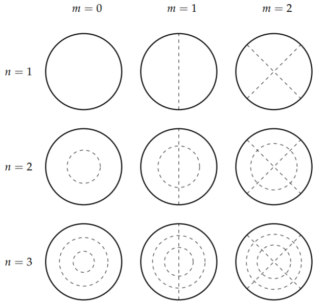
For the angular part, we easily see that the nodal curves are radial lines, \(θ =\text{const}\). For \(m = 0\), there are no solutions, since \(\cos mθ = 1\) for \(m = 0\). in Figure \(\PageIndex{2}\) this is seen by the absence of radial lines in the first column.
For \(m=1\), we have \(\cos \theta=0\). This implies that \(\theta=\pm \frac{\pi}{2}\). These values give the vertical line as shown in the second column in Figure \(\PageIndex{2}\). For \(m=2, \cos 2 \theta=0\) implies that \(\theta=\frac{\pi}{4}, \frac{3 \pi}{4}\). This results in the two lines shown in the last column of Figure \(\PageIndex{2}\).
We can also consider the nodal curves defined by the Bessel functions. We seek values of \(r\) for which \(\frac{j m m}{a} r\) is a zero of the Bessel function and lies in the interval \([0, a]\). Thus, we have
\[\frac{j_{m n}}{a} r=j_{m j}, \quad 1 \leq j \leq n,\nonumber \]
or
\[r=\frac{j_{m j}}{j_{m n}} a, \quad 1 \leq j \leq n .\nonumber \]
These will give circles of these radii with \(j_{m j} \leq j_{m n}\), or \(j \leq n\). For \(m=0\) and \(n=1\), there is only one zero and \(r=a\). In fact, for all \(n=1\) modes, there is only one zero giving \(r=a\). Thus, the first row in Figure \(\PageIndex{2}\) shows no interior nodal circles.
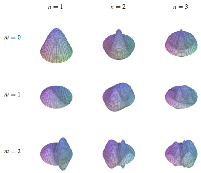
For a three dimensional view, one can look at Figure 6.1.3. Imagine that the various regions are oscillating independently and that the points on the nodal curves are not moving.
We should note that the nodal circles are not evenly spaced and that the radii can be computed relatively easily. For the \(n=2\) modes, we have two circles, \(r=a\) and \(r=\frac{j_{m 1}}{j_{m 2}} a\) as shown in the second row of Figure \(\PageIndex{2}\). For
Table \(\PageIndex{2}\): A three dimensional view of the vibrating circular membrane for the lowest modes. Compare these images with the nodal line plots in Figure \(\PageIndex{2}\).
\(m=0\),
\[r=\frac{2.405}{5.520}a\approx 0.4357a\nonumber \]
for the inner circle. For \(m=1\),
\[r=\frac{3.832}{7.016}a\approx 0.5462a,\nonumber \]
and for \(m=2\),
\[r=\frac{5.136}{8.417}a\approx 0.6102a.\nonumber \]
For \(n=3\) we obtain circles of radii
\[r=a,\quad r=\frac{j_{m1}}{j_{m3}}a,\quad\text{and}\quad r=\frac{j_{m2}}{j_{m3}}a.\nonumber \]
For \(m=0\),
\[r=a,\quad\frac{5.520}{8.654}a\approx 0.6379a,\quad\frac{2.405}{8.654}a\approx 0.2779a.\nonumber \]
Similarly, for \(m=1\),
\[r=a,\quad\frac{3.832}{10.173}a\approx 0.3767a,\quad\frac{7.016}{10.173}a\approx 0.6897a,\nonumber \]
and for \(m=2\),
\[r=a,\quad\frac{5.136}{11.620}a\approx 0.4420a,\quad\frac{8.417}{11.620}a\approx 0.7224a.\nonumber \]
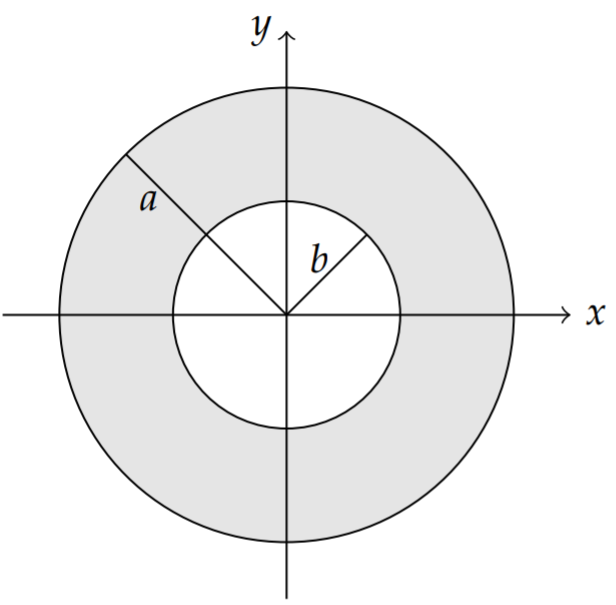
More complicated vibrations can be dreamt up for this geometry. Consider an annulus in which the drum is formed from two concentric circular cylinders and the membrane is stretch between the two with an annular cross section as shown in Figure \(\PageIndex{3}\). The separation would follow as before except now the boundary conditions are that the membrane is fixed around the two circular boundaries. In this case we cannot toss out the Neumann functions because the origin is not part of the drum head.
Solution
The domain for this problem is shown in Figure \(\PageIndex{3}\) and the problem is given by the partial differential equation
\[\begin{align} &u_{t t}=c^{2}\left[\frac{1}{r} \frac{\partial}{\partial r}\left(r \frac{\partial u}{\partial r}\right)+\frac{1}{r^{2}} \frac{\partial^{2} u}{\partial \theta^{2}}\right],\label{eq:14} \\ &t>0, \quad b<r<a, \quad-\pi<\theta<\pi, \end{align} \nonumber \]
the boundary conditions,
\[u(b, \theta, t)=0, \quad u(a, \theta, t)=0, \quad t>0, \quad-\pi<\theta<\pi,\label{eq:15} \]
and the initial conditions,
\[\begin{align} u(r, \theta, 0) &=f(r, \theta), \quad b<r<a,-\pi<\theta<\pi,\nonumber \\ u_{t}(r, \theta, 0) &=g(r, \theta), \quad \quad b<r<a,-\pi<\theta<\pi .\label{eq:16} \end{align} \]
Since we cannot dispose of the Neumann functions, the product solutions take the form
\[u(r, \theta, t)=\left\{\begin{array}{c} \cos \omega t \\ \sin \omega t \end{array}\right\}\left\{\begin{array}{c} \cos m \theta \\ \sin m \theta \end{array}\right\} R_{m}(r),\label{eq:17} \]
where
\[R_{m}(r)=c_{1} J_{m}(\sqrt{\lambda} r)+c_{2} N_{m}(\sqrt{\lambda} r)\nonumber \]
and \(\omega=c \sqrt{\lambda}, \quad m=0,1, \ldots\)
For this problem the radial boundary conditions are that the membrane is fixed at \(r=a\) and \(r=b\). Taking \(b<a\), we then have to satisfy the conditions
\[\begin{align} &R(a)=c_{1} J_{m}(\sqrt{\lambda} a)+c_{2} N_{m}(\sqrt{\lambda} a)=0,\nonumber \\ &R(b)=c_{1} J_{m}(\sqrt{\lambda} b)+c_{2} N_{m}(\sqrt{\lambda} b)=0 .\label{eq:18} \end{align} \]
This leads to two homogeneous equations for \(c_{1}\) and \(c_{2}\). The coefficient determinant of this system has to vanish if there are to be nontrivial solutions. This gives the eigenvalue equation for \(\lambda\) :
\[J_{m}(\sqrt{\lambda} a) N_{m}(\sqrt{\lambda} b)-J_{m}(\sqrt{\lambda} b) N_{m}(\sqrt{\lambda} a)=0 .\nonumber \]
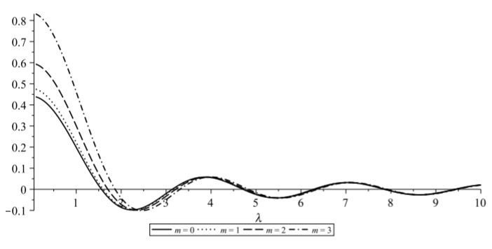
There are an infinite number of zeros of the function
\[F(\lambda)=\lambda: J_{m}(\sqrt{\lambda} a) N_{m}(\sqrt{\lambda} b)-J_{m}(\sqrt{\lambda} b) N_{m}(\sqrt{\lambda} a)\nonumber \]
In Figure \(\PageIndex{4}\) we show a plot of \(F(\lambda)\) for \(a=4, b=2\) and \(m=0,1,2,3\).
This eigenvalue equation needs to be solved numerically. Choosing \(a=2\) and \(b=4\), we have for the first few modes
\[\begin{array}{rlr} \sqrt{\lambda_{m n}} & \approx 1.562,3.137,4.709, & m=0 \\ & \approx 1.598,3.156,4.722, & m=1 \\ & \approx 1.703,3.214,4.761, & m=2 . \end{array}\label{eq:19} \]
Note, since \(\omega_{m n}=c \sqrt{\lambda_{m n}}\), these numbers essentially give us the frequencies of oscillation.
For these particular roots, we can solve for \(c_{1}\) and \(c_{2}\) up to a multiplicative constant. A simple solution is to set
\[c_{1}=N_{m}\left(\sqrt{\lambda_{m n}} b\right), \quad c_{2}=J_{m}\left(\sqrt{\lambda_{m n}} b\right) .\nonumber \]
This leads to the basic modes of vibration,
\[R_{mn}(r)\Theta_m(\theta)=\cos m\theta\left(N_m(\sqrt{\lambda_{mn}}b)J_m(\sqrt{\lambda_{mn}}r)-J_m(\sqrt{\lambda_{mn}}b)N_m(\sqrt{\lambda_{mn}}r)\right),\nonumber \]
for \(m=0,1, \ldots\), and \(n=1,2, \ldots\). In Figure \(\PageIndex{1}\) we show various modes for the particular choice of annular membrane dimensions, \(a=2\) and \(b=4\).