2.7: d’Alembert’s Solution of the Wave Equation

A general solution of the one-dimensional wave equation can be found. This solution was first Jean-Baptiste le Rond d’Alembert (1717- 1783) and is referred to as d’Alembert’s formula. In this section we will derive d’Alembert’s formula and then use it to arrive at solutions to the wave equation on infinite, semi-infinite, and finite intervals.

We consider the wave equation in the form \(u_{tt} = c^2u_{xx}\) and introduce the transformation

\[u(x,t)=U(\xi ,\eta),\quad\text{where}\quad\xi=x+ct\quad\text{and}\quad\eta=x-ct.\nonumber\]

Note that \(ξ\), and \(η\) are the characteristics of the wave equation.

We also need to note how derivatives transform. For example

\[\begin{align}\frac{\partial u}{\partial x}&=\frac{\partial U(\xi, \eta)}{\partial x} \nonumber \\ &=\frac{\partial U(\xi, \eta)}{\partial\xi}\frac{\partial\xi}{\partial x}+\frac{\partial U(\xi,\eta)}{\partial\eta}\frac{\partial\eta}{\partial x}\nonumber \\ &=\frac{\partial U(\xi,\eta)}{\partial\xi}+\frac{\partial U(\xi,\eta)}{\partial\eta}.\label{eq:1}\end{align}\]

Therefore, as an operator, we have

\[\frac{\partial}{\partial x}=\frac{\partial}{\partial\xi}+\frac{\partial}{\partial\eta}.\nonumber\]

Similarly, one can show that

\[\frac{\partial}{\partial t}=c\frac{\partial}{\partial\xi}-c\frac{\partial}{\partial\eta}.\nonumber\]

Using these results, the wave equation becomes

\[\begin{align}0&=u_{tt}-c^2u_{xx}\nonumber \\ &=\left(\frac{\partial^2}{\partial t^2}-c^2\frac{\partial^2}{\partial x^2}\right)u\nonumber \\ &=\left(\frac{\partial}{\partial t}+c\frac{\partial}{\partial x}\right)\left(\frac{\partial}{\partial t}-c\frac{\partial}{\partial x}\right)u\nonumber \\ &=\left(c\frac{\partial}{\partial\xi}-c\frac{\partial}{\partial\eta}+c\frac{\partial}{\partial\xi}+c\frac{\partial}{\partial\eta}\right)\left(c\frac{\partial}{\partial\xi}-c\frac{\partial}{\partial\eta}-c\frac{\partial}{\partial\xi}-c\frac{\partial}{\partial\eta}\right)U\nonumber \\ &=-4c^2\frac{\partial}{\partial\xi}\frac{\partial}{\partial\eta}U.\label{eq:2}\end{align}\]

Therefore, the wave equation has transformed into the simpler equation,

\[U_{\eta\xi}=0.\nonumber\]

A further integration gives

\[U(\xi ,\eta)=\int^\eta \Gamma (\eta ')d\eta '+F(\xi)=G(\eta)+F(\eta).\nonumber\]

Therefore, we have as the general solution of the wave equation,

\[\label{eq:3}u(x,t)=F(x+ct)+G(x-ct),\]

where \(F\) and \(G\) are two arbitrary, twice differentiable functions. As \(t\) is increased, we see that \(F(x + ct)\) gets horizontally shifted to the left and \(G(x − ct)\) gets horizontally shifted to the right. As a result, we conclude that the solution of the wave equation can be seen as the sum of left and right traveling waves.

Let’s use initial conditions to solve for the unknown functions. We let

\[u(x,0)=f(x),\quad u_t(x,0)=g(x),\quad |x|<\infty .\nonumber\]

Applying this to the general solution, we have

\[\begin{align}f(x)&=F(x)+G(x)\label{eq:4} \\ g(x)&=c[F'(x)-G'x)].\label{eq:5}\end{align}\]

We need to solve for \(F(x)\) and \(G(x)\) in terms of \(f(x)\) and \(g(x)\). Integrating Equation \(\eqref{eq:5}\), we have

\[\frac{1}{c}\int_0^x g(s)dx=F(x)-G(x)-F(0)+G(0).\nonumber\]

Adding this result to Equation \(\eqref{eq:5}\), gives

\[F(x)=\frac{1}{2}f(x)+\frac{1}{2c}\int_0^xg(s)ds+\frac{1}{2}[F(0)-G(0)].\nonumber\]

Subtracting from Equation \(\eqref{eq:5}\), gives

\[G(x)=\frac{1}{2}f(x)-\frac{1}{2c}\int_0^x g(s)ds-\frac{1}{2}[F(0)-G(0)].\nonumber\]

Now we can write out the solution \(u(x, t) = F(x + ct) + G(x − ct)\), yielding d’Alembert’s solution

\[\label{eq:6}u(x,t)=\frac{1}{2}[f(x+ct)+f(x-ct)]+\frac{1}{2c}\int_{x-ct}^{x+ct}g(s)ds.\]

When \(f(x)\) and \(g(x)\) are defined for all \(x ∈ R\), the solution is well-defined. However, there are problems on more restricted domains. In the next examples we will consider the semi-infinite and finite length string problems.In each case we will need to consider the domain of dependence and the domain of influence of specific points. These concepts are shown in Figure \(\PageIndex{1}\). The domain of dependence of point P is red region. The point P depends on the values of \(u\) and \(u_t\) at points inside the domain. The domain of influence of P is the blue region. The points in the region are influenced by the values of \(u\) and \(u_t\) at P.

Figure \(\PageIndex{1}\): The domain of dependence of point P is red region. The point P depends on the values of \(u\) and \(u_t\) at points inside the domain. The domain of influence of P is the blue region. The points in the region are influenced by the values of \(u\) and \(u_t\) at P.

Example \(\PageIndex{1}\)

Use d’Alembert’s solution to solve

\[u_{tt}=c^2u_{xx},\quad u(x,0)=f(x),\quad u_t(x,0)=g(x),\quad 0\leq x<\infty.\nonumber\]

Solution

The d’Alembert solution is not well-defined for this problem because \(f(x − ct)\) is not defined for \(x − ct < 0\) for \(c\), \(t > 0\). There are similar problems for \(g(x)\). This can be seen by looking at the characteristics in the \(xt\)-plane. In Figure \(\PageIndex{2}\) there are characteristics emanating from the points marked by \(η_0\) and \(ξ_0\) that intersect in the domain \(x > 0\). The point of intersection of the blue lines have a domain of dependence entirely in the region \(x\), \(t > 0\), however the domain of dependence of point P reaches outside this region. Only characteristics \(ξ = x + ct\) reach point P, but characteristics \(η = x − ct\) do not. But, we need \(f(η)\) and \(g(x)\) for \(x < ct\) to form a solution.

Figure \(\PageIndex{2}\): The characteristics for the semi-infinite string.

This can be remedied if we specified boundary conditions at \(x = 0\). For example, Fixed end boundary condition we will assume the end \(x = 0\) is fixed,

\[u(0,t)=0,\quad t\geq 0.\nonumber\]

Imagine an infinite string with one end (at \(x = 0\)) tied to a pole.

Since \(u(x, t) = F(x + ct) + G(x − ct)\), we have

\[u(0, t) = F(ct) + G(−ct) = 0.\nonumber\]

Letting \(ζ = −ct\), this gives \(G(ζ) = −F(−ζ),\) \(ζ ≤ 0\).

Note that

\[\begin{align} G(ζ) &=\frac{1}{2} f(ζ)-\frac{1}{2c}\int_0^ζ g(s)ds \nonumber \\ -F(-ζ)&=-\frac{1}{2}f(-ζ)-\frac{1}{2c}\int_0^{-ζ}g(s)ds\nonumber \\ &=-\frac{1}{2}f(-ζ)+\frac{1}{2c}\int_0^ζ g(\sigma )d\sigma \label{eq:7}\end{align}\]

Comparing the expressions for \(G(ζ)\) and \(−F(−ζ)\), we see that

\[f(ζ)=-f(-ζ),\quad g(ζ)=-g(-ζ).\nonumber\]

These relations imply that we can extend the functions into the region \(x < 0\) if we make them odd functions, or what are called odd extensions. An example is shown in Figure \(\PageIndex{3}\).

Another type of boundary condition is if the end \(x = 0\) is free,

\[u_x(0,t)=0,\quad t\geq 0.\nonumber\]

In this case we could have an infinite string tied to a ring and that ring is allowed to slide freely up and down a pole.

One can prove that this leads to

\[f(-\xi)=f(\xi),\quad g(-\xi)=g(\xi).\nonumber\]

Thus, we can use an even extension of these function to produce solutions.

Example \(\PageIndex{2}\)

Solve the initial-boundary value problem

\[\begin{align} u_{tt}&=c^2u_{xx},\quad 0\leq x<\infty ,\quad t>0.\nonumber \\ u(x,0)&=\left\{\begin{array}{ccc}x,& 0\leq x\leq 1, \\ 2-x, & 1\leq x\leq 2,& 0\leq x<\infty \\ 0,& x>2,\end{array}\right. \nonumber \\ u_t(x,0)&=0,\quad 0\leq x<\infty .\nonumber \\ u(0,t)&=0,\quad t>0.\label{eq:8}\end{align}\]

Solution

This is a semi-infinite string with a fixed end. Initially it is plucked to produce a nonzero triangular profile for \(0 ≤ x ≤ 2\). Since the initial velocity is zero, the general solution is found from d’Alembert’s solution,

\[u(x,t)=\frac{1}{2}[f_0(x+ct)+f_0(x-ct)],\nonumber\]

where \(f_0(x)\) is the odd extension of \(f(x) = u(x, 0)\). In Figure \(\PageIndex{3}\) we show the initial condition and its odd extension. The odd extension is obtained through reflection of \(f(x)\) about the origin.

Figure \(\PageIndex{3}\): The initial condition and its odd extension. The odd extension is obtained through reflection of \(f(x)\) about the origin.

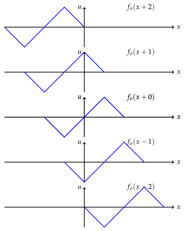
The next step is to look at the horizontal shifts of \(f_0(x)\). Several examples are shown in Figure \(\PageIndex{4}\).These show the left and right traveling waves.

Figure \(\PageIndex{4}\): Examples of \(f_0(x+ct)\) and \(f_0(x-ct)\).

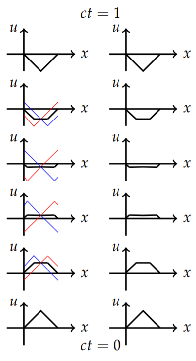
In Figure \(\PageIndex{5}\) we show superimposed plots of \(f_0(x + ct)\) and \(f_0(x − ct)\) for given times. The initial profile in at the bottom. By the time \(ct = 2\) the full traveling wave has emerged. The solution to the problem emerges on the right side of the figure by averaging each plot.

Figure \(\PageIndex{5}\): Superimposed plots of \(f_0(x + ct)\) and \(f_0(x − ct)\) for given times. The initial profile in at the bottom. By the time \(ct = 2\) the full traveling wave has emerged.

Figure \(\PageIndex{6}\): On the left is a plot of \(f(x + ct)\), \(f(x − ct)\) from Figure \(\PageIndex{5}\) and the average, \(u(x, t)\). On the right the solution alone is shown for \(ct = 0\) at bottom to \(ct = 1\) at top for the semi-infinite string problem

Example \(\PageIndex{3}\)

Use d’Alembert’s solution to solve

\[u_{tt}=c^2u_{xx},\quad u(x,0)=f(x),\quad u_t(x,0)=g(x),\quad 0\leq x\leq\ell .\nonumber\]

Solution

The general solution of the wave equation was found in the form

\[u(x,t)=F(x+ct)+G(x-ct).\nonumber\]

However, for this problem we can only obtain information for values of \(x\) and \(t\) such that \(0 ≤ x + ct ≤\ell\) and \(0 ≤ x − ct ≤ \ell\). In Figure \(\PageIndex{7}\) the characteristics \(x = ξ + ct\) and \(x = η − ct\) for \(0 ≤ ξ\), \(η ≤ \ell\). The main (gray) triangle, which is the domain of dependence of the point \((\ell, 2, \ell /2c)\), is the only region in which the solution can be found based solely on the initial conditions. As with the previous problem, boundary conditions will need to be given in order to extend the domain of the solution.

Figure \(\PageIndex{7}\): The characteristics emanating from the interval \(0 ≤ x ≤\ell\) for the finite string problem.

In the last example we saw that a fixed boundary at \(x = 0\) could be satisfied when \(f(x)\) and \(g(x)\) are extended as odd functions. In Figure \(\PageIndex{8}\) we indicate how the characteristics are affected by drawing in the new one as red dashed lines. This allows us to now construct solutions based on the initial conditions under the line \(x = \ell − ct\) for \(0 ≤ x ≤ \ell\). The new region for which we can construct solutions from the initial conditions is indicated in gray in Figure \(\PageIndex{8}\).

Figure \(\PageIndex{8}\): The red dashed lines are the characteristics from the interval \([−\ell, 0]\) from using the odd extension about \(x = 0\).

We can add characteristics on the right by adding a boundary condition at \(x =\ell\). Again, we could use fixed \(u(\ell, t) = 0\), or free, \(u_x(\ell, t) = 0\), boundary conditions. This allows us to now construct solutions based on the initial conditions for \(\ell ≤ x ≤ 2\ell\).

Let’s consider a fixed boundary condition at \(x =\ell\). Then, the solution must satisfy

\[u(\ell ,t)=F(\ell +ct)+G(\ell -ct)=0.\nonumber\]

To see what this means, let \(ζ =\ell + ct\). Then, this condition gives (since \(ct = ζ −\ell\))

\[F(\xi )=-G(2\ell -\xi),\quad \ell\leq\xi\leq 2\ell .\nonumber\]

Note that \(G(2\ell − ζ)\) is defined for \(0 ≤ 2\ell − ζ ≤\ell\). Therefore, this is a well-defined extension of the domain of \(F(x)\).

Note that

\[\begin{align} F(\xi )&=\frac{1}{2}f(\xi )+\frac{1}{2c}\int_0^\ell g(s)ds.\nonumber \\ -G(2\ell -\xi )&=-\frac{1}{2}f(2\ell -\xi)+\frac{1}{2c}\int_0^{2\ell -\xi}g(s)ds\nonumber \\ &=-\frac{1}{2}f(2\ell -\xi)-\frac{1}{2c}\int_0^\xi g(2\ell -\sigma)d\sigma\label{eq:9}\end{align}\]

Comparing the expressions for \(G(ζ)\) and \(−G(2\ell − ζ)\), we see that

\[f(\xi )=-f(2\ell -\xi),\quad g(\xi)=-g(2\ell -\xi).\nonumber\]

These relations imply that we can extend the functions into the region \(x >\ell\) if we consider an odd extension of \(f(x)\) and \(g(x)\) about \(x =\ell\). This will give the blue dashed characteristics in Figure \(\PageIndex{9}\) and a larger gray region to construct the solution.

Figure \(\PageIndex{9}\): The red dashed lines are the characteristics from the interval \([−\ell, 0]\) from using the odd extension about \(x = 0\) and the blue dashed lines are the characteristics from the interval \([\ell, 2\ell]\) from using the odd extension about \(x =\ell\).

So far we have extended \(f(x)\) and \(g(x)\) to the interval \(−\ell ≤ x ≤ 2\ell\) in order to determine the solution over a larger \(xt\)-domain. For example, the function \(f(x)\) has been extended to

\[f_{ext}(x)=\left\{\begin{array}{cc}-f(-x), &-\ell <x<0, \\ f(x),& 0<x<\ell , \\ -f(2\ell -x),&\ell <x<2\ell .\end{array}\right.\nonumber\]

A similar extension is needed for \(g(x)\). Inserting these extended functions into d’Alembert’s solution, we can determine \(u(x, t)\) in the region indicated in Figure \(\PageIndex{9}\).

Even though the original region has been expanded, we have not determined how to find the solution throughout the entire strip, \([0, \ell] × [0, ∞)\). This is accomplished by periodically repeating these extended functions with period \(2\ell\). This can be shown from the two conditions

\[f(x)=-f(-x),\quad -\ell\leq x\leq 0,\nonumber\]

\[\label{eq:10}f(x)=-f(2\ell -x),\quad\ell\leq x\leq 2\ell.\]

Now, consider

\[\begin{align} f(x+2\ell )&=-f(2\ell -(x-2\ell ))\nonumber \\ &=-f(-x)\nonumber \\ &=f(x).\label{eq:11}\end{align}\]

This shows that \(f(x)\) is periodic with period \(2\ell\). Since \(g(x)\) satisfies the same conditions, then it is as well.

In Figure \(\PageIndex{10}\) we show how the characteristics are extended throughout the domain strip using the periodicity of the extended initial conditions. The characteristics from the interval endpoints zig zag throughout the domain, filling it up. In the next example we show how to construct the odd periodic extension of a specific function.

Figure \(\PageIndex{10}\): Extending the characteristics throughout the domain strip.

Example \(\PageIndex{4}\)

Construct the periodic extension of the plucked string initial profile given by

\[f(x)=\left\{\begin{array}{cc}x,&0\leq x\leq\frac{\ell}{2}, \\ \ell -x,&\frac{\ell}{2}\leq x\leq\ell ,\end{array}\right.\nonumber\]

satisfying fixed boundary conditions at \(x = 0\) and \(x =\ell\).

Solution

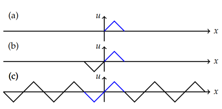
We first take the solution and add the odd extension about \(x = 0\). Then we add an extension beyond \(x =\ell\). This process is shown in Figure \(\PageIndex{11}\).

Figure \(\PageIndex{11}\): Construction of odd periodic extension for (a) The initial profile, \(f(x)\). (b) Make \(f(x)\) an odd function on \([−\ell,\ell ]\). (c) Make the odd function periodic with period \(2\ell\).

We can use the odd periodic function to construct solutions. In this case we use the result from the last example for obtaining the solution of the problem in which the initial velocity is zero, \(u(x, t) =\frac{1}{2} [ f(x + ct) + f(x − ct)]\). Translations of the odd periodic extension are shown in Figure \(\PageIndex{12}\).

Figure \(\PageIndex{12}\): Translations of the odd periodic extension.

In Figure \(\PageIndex{13}\) we show superimposed plots of \(f(x + ct)\) and \(f(x − ct)\) for different values of \(ct\). A box is shown inside which the physical wave can be constructed. The solution is an average of these odd periodic extensions within this box. This is displayed in Figure \(\PageIndex{14}\).

Figure \(\PageIndex{13}\): Superimposed translations of the odd periodic extension.

Figure \(\PageIndex{14}\): On the left is a plot of \(f(x + ct)\), \(f(x − ct)\) from Figure \(\PageIndex{13}\) and the average, \(u(x, t)\). On the right the solution alone is shown for \(ct = 0\) to \(ct = 1\).