
10.1: Ordinary Differential Equations
- Page ID
- 90282

\( \newcommand{\vecs}[1]{\overset { \scriptstyle \rightharpoonup} {\mathbf{#1}} } \)
\( \newcommand{\vecd}[1]{\overset{-\!-\!\rightharpoonup}{\vphantom{a}\smash {#1}}} \)
\( \newcommand{\dsum}{\displaystyle\sum\limits} \)
\( \newcommand{\dint}{\displaystyle\int\limits} \)
\( \newcommand{\dlim}{\displaystyle\lim\limits} \)
\( \newcommand{\id}{\mathrm{id}}\) \( \newcommand{\Span}{\mathrm{span}}\)
( \newcommand{\kernel}{\mathrm{null}\,}\) \( \newcommand{\range}{\mathrm{range}\,}\)
\( \newcommand{\RealPart}{\mathrm{Re}}\) \( \newcommand{\ImaginaryPart}{\mathrm{Im}}\)
\( \newcommand{\Argument}{\mathrm{Arg}}\) \( \newcommand{\norm}[1]{\| #1 \|}\)
\( \newcommand{\inner}[2]{\langle #1, #2 \rangle}\)
\( \newcommand{\Span}{\mathrm{span}}\)
\( \newcommand{\id}{\mathrm{id}}\)
\( \newcommand{\Span}{\mathrm{span}}\)
\( \newcommand{\kernel}{\mathrm{null}\,}\)
\( \newcommand{\range}{\mathrm{range}\,}\)
\( \newcommand{\RealPart}{\mathrm{Re}}\)
\( \newcommand{\ImaginaryPart}{\mathrm{Im}}\)
\( \newcommand{\Argument}{\mathrm{Arg}}\)
\( \newcommand{\norm}[1]{\| #1 \|}\)
\( \newcommand{\inner}[2]{\langle #1, #2 \rangle}\)
\( \newcommand{\Span}{\mathrm{span}}\) \( \newcommand{\AA}{\unicode[.8,0]{x212B}}\)
\( \newcommand{\vectorA}[1]{\vec{#1}} % arrow\)
\( \newcommand{\vectorAt}[1]{\vec{\text{#1}}} % arrow\)
\( \newcommand{\vectorB}[1]{\overset { \scriptstyle \rightharpoonup} {\mathbf{#1}} } \)
\( \newcommand{\vectorC}[1]{\textbf{#1}} \)
\( \newcommand{\vectorD}[1]{\overrightarrow{#1}} \)
\( \newcommand{\vectorDt}[1]{\overrightarrow{\text{#1}}} \)
\( \newcommand{\vectE}[1]{\overset{-\!-\!\rightharpoonup}{\vphantom{a}\smash{\mathbf {#1}}}} \)
\( \newcommand{\vecs}[1]{\overset { \scriptstyle \rightharpoonup} {\mathbf{#1}} } \)
\(\newcommand{\longvect}{\overrightarrow}\)
\( \newcommand{\vecd}[1]{\overset{-\!-\!\rightharpoonup}{\vphantom{a}\smash {#1}}} \)
\(\newcommand{\avec}{\mathbf a}\) \(\newcommand{\bvec}{\mathbf b}\) \(\newcommand{\cvec}{\mathbf c}\) \(\newcommand{\dvec}{\mathbf d}\) \(\newcommand{\dtil}{\widetilde{\mathbf d}}\) \(\newcommand{\evec}{\mathbf e}\) \(\newcommand{\fvec}{\mathbf f}\) \(\newcommand{\nvec}{\mathbf n}\) \(\newcommand{\pvec}{\mathbf p}\) \(\newcommand{\qvec}{\mathbf q}\) \(\newcommand{\svec}{\mathbf s}\) \(\newcommand{\tvec}{\mathbf t}\) \(\newcommand{\uvec}{\mathbf u}\) \(\newcommand{\vvec}{\mathbf v}\) \(\newcommand{\wvec}{\mathbf w}\) \(\newcommand{\xvec}{\mathbf x}\) \(\newcommand{\yvec}{\mathbf y}\) \(\newcommand{\zvec}{\mathbf z}\) \(\newcommand{\rvec}{\mathbf r}\) \(\newcommand{\mvec}{\mathbf m}\) \(\newcommand{\zerovec}{\mathbf 0}\) \(\newcommand{\onevec}{\mathbf 1}\) \(\newcommand{\real}{\mathbb R}\) \(\newcommand{\twovec}[2]{\left[\begin{array}{r}#1 \\ #2 \end{array}\right]}\) \(\newcommand{\ctwovec}[2]{\left[\begin{array}{c}#1 \\ #2 \end{array}\right]}\) \(\newcommand{\threevec}[3]{\left[\begin{array}{r}#1 \\ #2 \\ #3 \end{array}\right]}\) \(\newcommand{\cthreevec}[3]{\left[\begin{array}{c}#1 \\ #2 \\ #3 \end{array}\right]}\) \(\newcommand{\fourvec}[4]{\left[\begin{array}{r}#1 \\ #2 \\ #3 \\ #4 \end{array}\right]}\) \(\newcommand{\cfourvec}[4]{\left[\begin{array}{c}#1 \\ #2 \\ #3 \\ #4 \end{array}\right]}\) \(\newcommand{\fivevec}[5]{\left[\begin{array}{r}#1 \\ #2 \\ #3 \\ #4 \\ #5 \\ \end{array}\right]}\) \(\newcommand{\cfivevec}[5]{\left[\begin{array}{c}#1 \\ #2 \\ #3 \\ #4 \\ #5 \\ \end{array}\right]}\) \(\newcommand{\mattwo}[4]{\left[\begin{array}{rr}#1 \amp #2 \\ #3 \amp #4 \\ \end{array}\right]}\) \(\newcommand{\laspan}[1]{\text{Span}\{#1\}}\) \(\newcommand{\bcal}{\cal B}\) \(\newcommand{\ccal}{\cal C}\) \(\newcommand{\scal}{\cal S}\) \(\newcommand{\wcal}{\cal W}\) \(\newcommand{\ecal}{\cal E}\) \(\newcommand{\coords}[2]{\left\{#1\right\}_{#2}}\) \(\newcommand{\gray}[1]{\color{gray}{#1}}\) \(\newcommand{\lgray}[1]{\color{lightgray}{#1}}\) \(\newcommand{\rank}{\operatorname{rank}}\) \(\newcommand{\row}{\text{Row}}\) \(\newcommand{\col}{\text{Col}}\) \(\renewcommand{\row}{\text{Row}}\) \(\newcommand{\nul}{\text{Nul}}\) \(\newcommand{\var}{\text{Var}}\) \(\newcommand{\corr}{\text{corr}}\) \(\newcommand{\len}[1]{\left|#1\right|}\) \(\newcommand{\bbar}{\overline{\bvec}}\) \(\newcommand{\bhat}{\widehat{\bvec}}\) \(\newcommand{\bperp}{\bvec^\perp}\) \(\newcommand{\xhat}{\widehat{\xvec}}\) \(\newcommand{\vhat}{\widehat{\vvec}}\) \(\newcommand{\uhat}{\widehat{\uvec}}\) \(\newcommand{\what}{\widehat{\wvec}}\) \(\newcommand{\Sighat}{\widehat{\Sigma}}\) \(\newcommand{\lt}{<}\) \(\newcommand{\gt}{>}\) \(\newcommand{\amp}{&}\) \(\definecolor{fillinmathshade}{gray}{0.9}\)Euler’s Method
In this section we will look at the simplest method for solving first order equations, Euler’s Method. While it is not the most efficient method, it does provide us with a picture of how one proceeds and can be improved by introducing better techniques, which are typically covered in a numerical analysis text.
Let’s consider the class of first order initial value problems of the form
\[\frac{d y}{d x}=f(x, y), \quad y\left(x_{0}\right)=y_{0} .\label{eq:1} \]
We are interested in finding the solution \(y(x)\) of this equation which passes through the initial point \(\left(x_{0}, y_{0}\right)\) in the \(x y\)-plane for values of \(x\) in the interval \([a, b]\), where \(a=x_{0}\). We will seek approximations of the solution at \(N\) points, labeled \(x_{n}\) for \(n=1, \ldots, N\). For equally spaced points we have \(\Delta x=x_{1}-x_{0}=x_{2}-x_{1}\), etc. We can write these as
\[x_{n}=x_{0}+n \Delta x .\nonumber \]
In Figure \(\PageIndex{1}\) we show three such points on the \(x\)-axis.
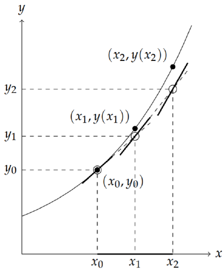
The first step of Euler’s Method is to use the initial condition. We represent this as a point on the solution curve, \(\left(x_{0}, y\left(x_{0}\right)\right)=\left(x_{0}, y_{0}\right)\), as shown in Figure \(\PageIndex{1}\). The next step is to develop a method for obtaining approximations to the solution for the other \(x_{n}\) ’s.
We first note that the differential equation gives the slope of the tangent line at \((x, y(x))\) of the solution curve since the slope is the derivative, \(y^{\prime}(x)^{\prime}\) From the differential equation the slope is \(f(x, y(x))\). Referring to Figure \(\PageIndex{1}\), we see the tangent line drawn at \(\left(x_{0}, y_{0}\right)\). We look now at \(x=x_{1}\). The vertical line \(x=x_{1}\) intersects both the solution curve and the tangent line passing through \(\left(x_{0}, y_{0}\right)\). This is shown by a heavy dashed line.
While we do not know the solution at \(x=x_{1}\), we can determine the tangent line and find the intersection point that it makes with the vertical. As seen in the figure, this intersection point is in theory close to the point on the solution curve. So, we will designate \(y_{1}\) as the approximation of the solution \(y\left(x_{1}\right)\). We just need to determine \(y_{1}\).
The idea is simple. We approximate the derivative in the differential equation by its difference quotient:
\[\frac{d y}{d x} \approx \frac{y_{1}-y_{0}}{x_{1}-x_{0}}=\frac{y_{1}-y_{0}}{\Delta x} .\label{eq:2} \]
Since the slope of the tangent to the curve at \(\left(x_{0}, y_{0}\right)\) is \(y^{\prime}\left(x_{0}\right)=f\left(x_{0}, y_{0}\right)\), we can write
\[\frac{y_{1}-y_{0}}{\Delta x} \approx f\left(x_{0}, y_{0}\right) .\label{eq:3} \]
Solving this equation for \(y_{1}\), we obtain
\[y_{1}=y_{0}+\Delta x f\left(x_{0}, y_{0}\right) .\label{eq:4} \]
This gives \(y_{1}\) in terms of quantities that we know.
We now proceed to approximate \(y\left(x_{2}\right)\). Referring to Figure \(\PageIndex{1}\), we see that this can be done by using the slope of the solution curve at \(\left(x_{1}, y_{1}\right)\). The corresponding tangent line is shown passing though \(\left(x_{1}, y_{1}\right)\) and we can then get the value of \(y_{2}\) from the intersection of the tangent line with a vertical line, \(x=x_{2}\). Following the previous arguments, we find that
\[y_{2}=y_{1}+\Delta x f\left(x_{1}, y_{1}\right) .\label{eq:5} \]
Continuing this procedure for all \(x_{n}, n=1, \ldots N\), we arrive at the following scheme for determining a numerical solution to the initial value problem:
\[\begin{align} &y_{0}=y\left(x_{0}\right),\nonumber \\ &y_{n}=y_{n-1}+\Delta x f\left(x_{n-1}, y_{n-1}\right), \quad n=1, \ldots, N .\label{eq:6} \end{align} \]
This is referred to as Euler’s Method.
Use Euler’s Method to solve the initial value problem \(\frac{d y}{d x}=x+\) \(y, \quad y(0)=1\) and obtain an approximation for \(y(1)\).
Solution
First, we will do this by hand. We break up the interval \([0,1]\), since we want the solution at \(x=1\) and the initial value is at \(x=0\). Let \(\Delta x=0.50\). Then, \(x_{0}=0\), \(x_{1}=0.5\) and \(x_{2}=1.0\). Note that there are \(N=\frac{b-a}{\Delta x}=2\) subintervals and thus three points.
We next carry out Euler’s Method systematically by setting up a table for the needed values. Such a table is shown in Table \(\PageIndex{1}\). Note how the table is set up. There is a column for each \(x_{n}\) and \(y_{n}\). The first row is the initial condition. We also made use of the function \(f(x, y)\) in computing the \(y_{n}\) ’s from \(\eqref{eq:6}\). This sometimes makes the computation easier. As a result, we find that the desired approximation is given as \(y_{2}=2.5\).
| \(n\) | \(x_{n}\) | \(y_{n}=y_{n-1}+\Delta x f\left(x_{n-1}, y_{n-1}=0.5 x_{n-1}+1.5 y_{n-1}\right.\) |
|---|---|---|
| \(\mathrm{o}\) | \(\mathrm{o}\) | 1 |
| 1 | \(\mathrm{o} .5\) | \(0.5(0)+1.5(1.0)=1.5\) |
| 2 | \(1 . \mathrm{o}\) | \(0.5(0.5)+1.5(1.5)=2.5\) |
Is this a good result? Well, we could make the spatial increments smaller. Let’s repeat the procedure for \(\Delta x=0.2\), or \(N=5\). The results are in Table \(\PageIndex{2}\).
Now we see that the approximation is \(y_{1}=2.97664\). So, it looks like the value is near 3, but we cannot say much more. Decreasing \(\Delta x\) more shows that we are beginning to converge to a solution. We see this in Table \(\PageIndex{3}\).
| \(n\) | \(x_{n}\) | \(y_{n}=0.2 x_{n-1}+1.2 y_{n-1}\) |
|---|---|---|
| \(o\) | \(\circ\) | 1 |
| 1 | \(0.2\) | \(0.2(0)+1.2(1.0)=1.2\) |
| 2 | \(0.4\) | \(0.2(0.2)+1.2(1.2)=1.48\) |
| 3 | \(0.6\) | \(0.2(0.4)+1.2(1.48)=1.856\) |
| 4 | \(0.8\) | \(0.2(0.6)+1.2(1.856)=2.3472\) |
| 5 | \(1.0\) | \(0.2(0.8)+1.2(2.3472)=2.97664\) |
| \(\Delta x\) | \(y_{N} \approx y(1)\) |
|---|---|
| \(0.5\) | \(2.5\) |
| \(0.2\) | \(2.97664\) |
| \(0.1\) | \(3.187484920\) |
| \(0.01\) | \(3.409627659\) |
| \(0.001\) | \(3.433847864\) |
| \(0.0001\) | \(3.436291854\) |
Of course, these values were not done by hand. The last computation would have taken 1000 lines in the table, or at least 40 pages! One could use a computer to do this. A simple code in Maple would look like the following:
> restart:
> f:=(x,y)->y+x;
> a:=0: b:=1: N:=100: h:=(b-a)/N;
> x[0]:=0: y[0]:=1:
    for i from 1 to N do
    y[i]:=y[i-1]+h*f(x[i-1],y[i-1]):
    x[i]:=x[0]+h*(i):
    od:
    evalf(y[N]);
In this case we could simply use the exact solution. The exact solution is easily found as
\[y(x)=2 e^{x}-x-1 .\nonumber \]
(The reader can verify this.) So, the value we are seeking is
\[y(1)=2 e-2=3.4365636 \ldots .\nonumber \]
Thus, even the last numerical solution was off by about \(0.00027\).
Adding a few extra lines for plotting, we can visually see how well the approximations compare to the exact solution. The Maple code for doing such a plot is given below.
> with(plots):
> Data:=[seq([x[i],y[i]],i=0..N)]:
> P1:=pointplot(Data,symbol=DIAMOND):
> Sol:=t->-t-1+2*exp(t);
> P2:=plot(Sol(t),t=a..b,Sol=0..Sol(b)):
> display({P1,P2});
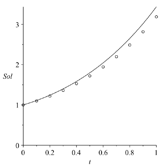
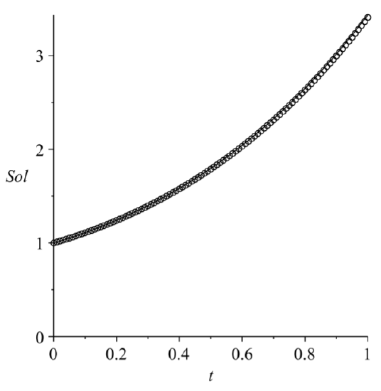
We show in Figures \(\PageIndex{2}\)-\(\PageIndex{3}\) the results for \(N = 10\) and \(N = 100\). In Figure \(\PageIndex{2}\) we can see how quickly the numerical solution diverges from the exact solution. In Figure \(\PageIndex{3}\) we can see that visually the solutions agree, but we note that from Table \(\PageIndex{3}\) that for \(∆x = 0.01\), the solution is still off in the second decimal place with a relative error of about \(0.8\)%.
Why would we use a numerical method when we have the exact solution? Exact solutions can serve as test cases for our methods. We can make sure our code works before applying them to problems whose solution is not known.
There are many other methods for solving first order equations. One commonly used method is the fourth order Runge-Kutta method. This method has smaller errors at each step as compared to Euler’s Method. It is well suited for programming and comes built-in in many packages like Maple and MATLAB. Typically, it is set up to handle systems of first order equations.
In fact, it is well known that \(n\)th order equations can be written as a system of \(n\) first order equations. Consider the simple second order equation
\[y^{\prime \prime}=f(x, y) \text {. }\nonumber \]
This is a larger class of equations than the second order constant coefficient equation. We can turn this into a system of two first order differential equations by letting \(u=y\) and \(v=y^{\prime}=u^{\prime}\). Then, \(v^{\prime}=y^{\prime \prime}=f(x, u)\). So, we have the first order system
\[\begin{align} &u^{\prime}=v\nonumber \\ &v^{\prime}=f(x, u) .\label{eq:7} \end{align} \]
We will not go further into the Runge-Kutta Method here. You can find more about it in a numerical analysis text. However, we will see that systems of differential equations do arise naturally in physics. Such systems are often coupled equations and lead to interesting behaviors.
Higher Order Taylor Methods
Euler's Method for solving differential equations is easy to understand but is not efficient in the sense that it is what is called a first order method. The error at each step, the local truncation error, is of order \(\Delta x\), for \(x\) the independent variable. The accumulation of the local truncation errors results in what is called the global error. In order to generalize Euler’s Method, we need to rederive it. Also, since these methods are typically used for initial value problems, we will cast the problem to be solved as
\[\frac{d y}{d t}=f(t, y), \quad y(a)=y_{0}, \quad t \in[a, b] .\label{eq:8} \]
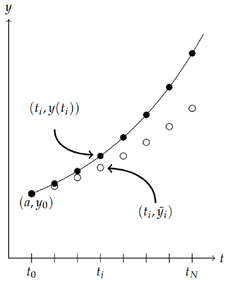
The first step towards obtaining a numerical approximation to the solution of this problem is to divide the \(t\)-interval, \([a, b]\), into \(N\) subintervals,
\[t_{i}=a+i h, \quad i=0,1, \ldots, N, \quad t_{0}=a, \quad t_{N}=b,\nonumber \]
where
\[h=\frac{b-a}{N} .\nonumber \]
We then seek the numerical solutions
\[\tilde{y}_{i} \approx y\left(t_{i}\right), \quad i=1,2, \ldots, N,\nonumber \]
with \(\tilde{y}_{0}=y\left(t_{0}\right)=y_{0}\). Figure \(\PageIndex{4}\) graphically shows how these quantities are related.
Euler’s Method can be derived using the Taylor series expansion of of the solution \(y\left(t_{i}+h\right)\) about \(t=t_{i}\) for \(i=1,2, \ldots, N\). This is given by
\[\begin{align} y\left(t_{i+1}\right) &=y\left(t_{i}+h\right)\nonumber \\ &=y\left(t_{i}\right)+y^{\prime}\left(t_{i}\right) h+\frac{h^{2}}{2} y^{\prime \prime}\left(\xi_{i}\right), \quad \xi_{i} \in\left(t_{i}, t_{i+1}\right) .\label{eq:9} \end{align} \]
Here the term \(\frac{h^{2}}{2} y^{\prime \prime}\left(\xi_{i}\right)\) captures all of the higher order terms and represents the error made using a linear approximation to \(y\left(t_{i}+h\right)\).
Dropping the remainder term, noting that \(y^{\prime}(t)=f(t, y)\), and defining the resulting numerical approximations by \(\tilde{y}_{i} \approx y\left(t_{i}\right)\), we have
\[\begin{align} \tilde{y}_{i+1} &=\tilde{y}_{i}+h f\left(t_{i}, \tilde{y}_{i}\right), \quad i=0,1, \ldots, N-1,\nonumber \\ \tilde{y}_{0} &=y(a)=y_{0} .\label{eq:10} \end{align} \]
This is Euler’s Method.
Euler’s Method is not used in practice since the error is of order \(h\). However, it is simple enough for understanding the idea of solving differential equations numerically. Also, it is easy to study the numerical error, which we will show next.
The error that results for a single step of the method is called the local truncation error, which is defined by
\[\tau_{i+1}(h)=\frac{y\left(t_{i+1}\right)-\tilde{y}_{i}}{h}-f\left(t_{i}, y_{i}\right) .\nonumber \]
A simple computation gives
\[\tau_{i+1}(h)=\frac{h}{2} y^{\prime \prime}\left(\xi_{i}\right), \quad \xi_{i} \in\left(t_{i}, t_{i+1}\right) .\nonumber \]
Since the local truncation error is of order \(h\), this scheme is said to be of order one. More generally, for a numerical scheme of the form
\[\begin{align} \tilde{y}_{i+1} &=\tilde{y}_{i}+h F\left(t_{i}, \tilde{y}_{i}\right), \quad i=0,1, \ldots, N-1,\nonumber \\ \tilde{y}_{0} &=y(a)=y_{0},\label{eq:11} \end{align} \]
the local truncation error is defined by
\[\tau_{i+1}(h)=\frac{y\left(t_{i+1}\right)-\tilde{y}_{i}}{h}-F\left(t_{i}, y_{i}\right) .\nonumber \]
The accumulation of these errors leads to the global error. In fact, one can show that if \(f\) is continuous, satisfies the Lipschitz condition,
\[\left|f\left(t, y_{2}\right)-f\left(t, y_{1}\right)\right| \leq L\left|y_{2}-y_{1}\right|\nonumber \]
for a particular domain \(D \subset R^{2}\), and
\[\left|y^{\prime \prime}(t)\right| \leq M, \quad t \in[a, b],\nonumber \]
then
\[\mid y\left(t_{i}\right)-\tilde{y}_{\mid} \leq \frac{h M}{2 L}\left(e^{L\left(t_{i}-a\right)}-1\right), \quad i=0,1, \ldots, N .\nonumber \]
Furthermore, if one introduces round-off errors, bounded by \(\delta\), in both the initial condition and at each step, the global error is modified as
\[\left|y\left(t_{i}\right)-\tilde{y}_{\mid} \leq \frac{1}{L}\left(\frac{h M}{2}+\frac{\delta}{h}\right)\left(e^{L\left(t_{i}-a\right)}-1\right)+\right| \delta_{0} \mid e^{L\left(t_{i}-a\right)}, \quad i=0,1, \ldots, N .\nonumber \]
Then for small enough steps \(h\), there is a point when the round-off error will dominate the error. [See Burden and Faires, Numerical Analysis for the details.]
Can we improve upon Euler’s Method? The natural next step towards finding a better scheme would be to keep more terms in the Taylor series expansion. This leads to Taylor series methods of order \(n\).
Taylor series methods of order \(n\) take the form
\[\begin{align} \tilde{y}_{i+1} &=\tilde{y}_{i}+h T^{(n)}\left(t_{i}, \tilde{y}_{i}\right), \quad i=0,1, \ldots, N-1,\nonumber \\ \tilde{y}_{0} &=y_{0},\label{eq:12} \end{align} \]
where we have defined
\[T^{(n)}(t, y)=y^{\prime}(t)+\frac{h}{2} y^{\prime \prime}(t)+\cdots+\frac{h^{(n-1)}}{n !} y^{(n)}(t) .\nonumber \]
However, since \(y^{\prime}(t)=f(t, y)\), we can write
\[T^{(n)}(t, y)=f(t, y)+\frac{h}{2} f^{\prime}(t, y)+\cdots+\frac{h^{(n-1)}}{n !} f^{(n-1)}(t, y) .\nonumber \]
We note that for \(n=1\), we retrieve Euler’s Method as a special case. We demonstrate a third order Taylor’s Method in the next example.
Apply the third order Taylor’s Method to
\[\frac{d y}{d t}=t+y, \quad y(0)=1\nonumber \]
and obtain an approximation for \(y(1)\) for \(h=0.1\).
Solution
The third order Taylor’s Method takes the form
\[\begin{align} \tilde{y}_{i+1} &=\tilde{y}_{i}+h T^{(3)}\left(t_{i}, \tilde{y}_{i}\right), \quad i=0,1, \ldots, N-1,\nonumber \\ \tilde{y}_{0} &=y_{0},\label{eq:13} \end{align} \]
where
\[T^{(3)}(t, y)=f(t, y)+\frac{h}{2} f^{\prime}(t, y)+\frac{h^{2}}{3 !} f^{\prime \prime}(t, y)\nonumber \]
and \(f(t, y)=t+y(t)\).
In order to set up the scheme, we need the first and second derivative of \(f(t, y)\) :
\[\begin{align} f^{\prime}(t, y) &=\frac{d}{d t}(t+y)\nonumber \\ &=1+y^{\prime}\nonumber \\ &=1+t+y\label{eq:14} \\ f^{\prime \prime}(t, y) &=\frac{d}{d t}(1+t+y) \\ &=1+y^{\prime}\nonumber \\ &=1+t+y\label{eq:15} \end{align} \]
Inserting these expressions into the scheme, we have
\[\begin{align} \tilde{y}_{i+1} &=\tilde{y}_{i}+h\left[\left(t_{i}+y_{i}\right)+\frac{h}{2}\left(1+t_{i}+y_{i}\right)+\frac{h^{2}}{3 !}\left(1+t_{i}+y_{i}\right)\right],\nonumber \\ &=\tilde{y}_{i}+h\left(t_{i}+y_{i}\right)+h^{2}\left(\frac{1}{2}+\frac{h}{6}\right)\left(1+t_{i}+y_{i}\right),\nonumber \\ \tilde{y}_{0} &=y_{0},\label{eq:16} \end{align} \]
for \(i=0,1, \ldots, N-1\).
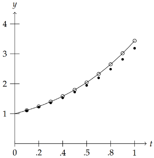
In Figure \(\PageIndex{2}\) we show the results comparing Euler’s Method, the 3rd Order Taylor’s Method, and the exact solution for \(N=10\). In Table \(\PageIndex{4}\) we provide are the numerical values. The relative error in Euler’s method is about \(7 \%\) and that of the 3rd Order Taylor’s Method is about \(0.006\%\). Thus, the 3rd Order Taylor’s Method is significantly better than Euler’s Method.
| Euler | Taylor | Exact |
|---|---|---|
| \(1.0000\) | \(1.0000\) | \(1.0000\) |
| \(1.1000\) | \(1.1103\) | \(1.1103\) |
| \(1.2200\) | \(1.2428\) | \(1.2428\) |
| \(1.3620\) | \(1.3997\) | \(1.3997\) |
| \(1.5282\) | \(1.5836\) | \(1.5836\) |
| \(1.7210\) | \(1.7974\) | \(1.7974\) |
| \(1.9431\) | \(2.0442\) | \(2.0442\) |
| \(2.1974\) | \(2.3274\) | \(2.3275\) |
| \(2.4872\) | \(2.6509\) | \(2.6511\) |
| \(2.8159\) | \(3.0190\) | \(3.0192\) |
| \(3.1875\) | \(3.4364\) | \(3.4366\) |
In the last section we provided some Maple code for performing Euler’s method. A similar code in MATLAB looks like the following:
a=0;
b=1;
N=10;
h=(b-a)/N;

% Slope function
    f = inline(’t+y’,’t’,’y’);
    sol = inline(’2*exp(t)-t-1’,’t’);

% Initial Condition
    t(1)=0;
    y(1)=1;

% Euler’s Method
    for i=2:N+1
        y(i)=y(i-1)+h*f(t(i-1),y(i-1));
        t(i)=t(i-1)+h;
    end
A simple modification can be made for the 3rd Order Taylor’s Method by replacing the Euler’s method part of the preceding code by
% Taylor’s Method, Order 3
    y(1)=1;
    h3 = h^2*(1/2+h/6);
    for i=2:N+1
        y(i)=y(i-1)+h*f(t(i-1),y(i-1))+h3*(1+t(i-1)+y(i-1));
        t(i)=t(i-1)+h;
    end
While the accuracy in the last example seemed sufficient, we have to remember that we only stopped at one unit of time. How can we be confident that the scheme would work as well if we carried out the computation for much longer times. For example, if the time unit were only a second, then one would need 86,400 times longer to predict a day forward. Of course, the scale matters. But, often we need to carry out numerical schemes for long times and we hope that the scheme not only converges to a solution, but that it converges to the solution to the given problem. Also, the previous example was relatively easy to program because we could provide a relatively simple form for \(T^{(3)}(t, y)\) with a quick computation of the derivatives of \(f(t, y)\). This is not always the case and higher order Taylor methods in this form are not typically used. Instead, one can approximate \(T^{(n)}(t, y)\) by evaluating the known function \(f(t, y)\) at selected values of \(t\) and \(y\), leading to Runge-Kutta methods.
Runge-Kutta Methods
As we had seen in the last section, we can use higher order Taylor methods to derive numerical schemes for solving
\[\frac{d y}{d t}=f(t, y), \quad y(a)=y_{0}, \quad t \in[a, b],\label{eq:17} \]
using a scheme of the form
\[\begin{align} \tilde{y}_{i+1} &=\tilde{y}_{i}+h T^{(n)}\left(t_{i}, \tilde{y}_{i}\right), \quad i=0,1, \ldots, N-1,\nonumber \\ \tilde{y}_{0} &=y_{0},\label{eq:18} \end{align} \]
where we have defined
\[T^{(n)}(t, y)=y^{\prime}(t)+\frac{h}{2} y^{\prime \prime}(t)+\cdots+\frac{h^{(n-1)}}{n !} y^{(n)}(t) .\nonumber \]
In this section we will find approximations of \(T^{(n)}(t, y)\) which avoid the need for computing the derivatives.
For example, we could approximate
\[T^{(2)}(t, y)=f(t, y)+\frac{h}{2} \operatorname{fracdfdt}(t, y)\nonumber \]
by
\[T^{(2)}(t, y) \approx a f(t+\alpha, y+\beta)\nonumber \]
for selected values of \(a, \alpha\), and \(\beta\). This requires use of a generalization of Taylor’s series to functions of two variables. In particular, for small \(\alpha\) and \(\beta\) we have
\[\begin{align} a f(t+\alpha, y+\beta)=& a\left[f(t, y)+\frac{\partial f}{\partial t}(t, y) \alpha+\frac{\partial f}{\partial y}(t, y) \beta\right.\nonumber \\ &\left.+\frac{1}{2}\left(\frac{\partial^{2} f}{\partial t^{2}}(t, y) \alpha^{2}+2 \frac{\partial^{2} f}{\partial t \partial y}(t, y) \alpha \beta+\frac{\partial^{2} f}{\partial y^{2}}(t, y) \beta^{2}\right)\right]\nonumber \\ &+\text { higher order terms. }\label{eq:19} \end{align} \]
Furthermore, we need \(\frac{d f}{d t}(t, y)\). Since \(y=y(t)\), this can be found using a generalization of the Chain Rule from Calculus III:
\[\frac{d f}{d t}(t, y)=\frac{\partial f}{\partial t}+\frac{\partial f}{\partial y} \frac{d y}{d t} .\nonumber \]
Thus,
\[T^{(2)}(t, y)=f(t, y)+\frac{h}{2}\left[\frac{\partial f}{\partial t}+\frac{\partial f}{\partial y} \frac{d y}{d t}\right] .\nonumber \]
Comparing this expression to the linear (Taylor series) approximation of af \((t+\alpha, y+\beta)\), we have
\[\begin{align} T^{(2)} & \approx a f(t+\alpha, y+\beta)\nonumber \\ f+\frac{h}{2} \frac{\partial f}{\partial t}+\frac{h}{2} f \frac{\partial f}{\partial y} & \approx a f+a \alpha \frac{\partial f}{\partial t}+\beta \frac{\partial f}{\partial y} .\label{eq:20} \end{align} \]
We see that we can choose
\[a=1, \quad \alpha=\frac{h}{2}, \quad \beta=\frac{h}{2} f .\nonumber \]
This leads to the numerical scheme
\[\begin{align} \tilde{y}_{i+1} &=\tilde{y}_{i}+h f\left(t_{i}+\frac{h}{2}, \tilde{y}_{i}+\frac{h}{2} f\left(t_{i}, \tilde{y}_{i}\right)\right), \quad i=0,1, \ldots, N-1,\nonumber \\ \tilde{y}_{0} &=y_{0},\label{eq:21} \end{align} \]
This Runge-Kutta scheme is called the Midpoint Method, or Second Order Runge-Kutta Method, and it has order 2 if all second order derivatives of \(f(t, y)\) are bounded.
Often, in implementing Runge-Kutta schemes, one computes the arguments separately as shown in the following MATLAB code snippet. (This code snippet could replace the Euler’s Method section in the code in the last section.)
% Midpoint Method
    y(1)=1;
    for i=2:N+1
        k1=h/2*f(t(i-1),y(i-1));
        k2=h*f(t(i-1)+h/2,y(i-1)+k1);
        y(i)=y(i-1)+k2;
        t(i)=t(i-1)+h;
    end
Compare the Midpoint Method with the 2nd Order Taylor’s Method for the problem
\[y^{\prime}=t^{2}+y, \quad y(0)=1, \quad t \in[0,1] .\label{eq:22} \]
Solution
The solution to this problem is \(y(t)=3 e^{t}-2-2 t-t^{2}\). In order to implement the 2nd Order Taylor’s Method, we need
\[\begin{align*} & T^{(2)} &=f(t, y)+\frac{h}{2} f^{\prime}(t, y)\nonumber \\ &=& t^{2}+y+\frac{h}{2}\left(2 t+t^{2}+y\right) .\label{eq:23} \end{align*} \]
The results of the implementation are shown in Table \(\PageIndex{3}\).
There are other way to approximate higher order Taylor polynomials. For example, we can approximate \(T^{(3)}(t, y)\) using four parameters by
\[T^{(3)}(t, y) \approx a f(t, y)+b f(t+\alpha, y+\beta f(t, y) .\nonumber \]
Expanding this approximation and using
\[T^{(3)}(t, y) \approx f(t, y)+\frac{h}{2} \frac{d f}{d t}(t, y)+\frac{h^{2}}{6} \frac{d f}{d t}(t, y),\nonumber \]
we find that we cannot get rid of \(O\left(h^{2}\right)\) terms. Thus, the best we can do is derive second order schemes. In fact, following a procedure similar to the derivation of the Midpoint Method, we find that
\[a+b=1, \quad, \alpha b=\frac{h}{2}, \beta=\alpha \text {. }\nonumber \]
There are three equations and four unknowns. Therefore there are many second order methods. Two classic methods are given by the modified Euler method \(\left(a=b=\frac{1}{2}, \alpha=\beta=h\right)\) and Huen’s method \(\left(a=\frac{1}{4}, b=\frac{3}{4}\right.\), \(\alpha=\beta=\frac{2}{3} h\).
| Exact | Taylor | Error | Midpoint | Error |
|---|---|---|---|---|
| \(1.0000\) | \(1.0000\) | \(0.0000\) | \(1.0000\) | \(0.0000\) |
| \(1.1055\) | \(1.1050\) | \(0.0005\) | \(1.1053\) | \(0.0003\) |
| \(1.2242\) | \(1.2231\) | \(0.0011\) | \(1.2236\) | \(0.0006\) |
| \(1.3596\) | \(1.3577\) | \(0.0019\) | \(1.3585\) | \(0.0010\) |
| \(1.5155\) | \(1.5127\) | \(0.0028\) | \(1.5139\) | \(0.0016\) |
| \(1.6962\) | \(1.6923\) | \(0.0038\) | \(1.6939\) | \(0.0023\) |
| \(1.9064\) | \(1.9013\) | \(0.0051\) | \(1.9032\) | \(0.0031\) |
| \(2.1513\) | \(2.1447\) | \(0.0065\) | \(2.1471\) | \(0.0041\) |
| \(2.4366\) | \(2.4284\) | \(0.0083\) | \(2.4313\) | \(0.0053\) |
| \(2.7688\) | \(2.7585\) | \(0.0103\) | \(2.7620\) | \(0.0068\) |
| \(3.1548\) | \(3.1422\) | \(0.0126\) | \(3.1463\) | \(0.0085\) |
The Fourth Order Runge-Kutta Method, which is most often used, is given by the scheme
\[\begin{aligned} \tilde{y}_{0} &=y_{0}, \\ k_{1} &=h f\left(t_{i}, \tilde{y}_{i}\right), \\ k_{2} &=h f\left(t_{i}+\frac{h}{2}, \tilde{y}_{i}+\frac{1}{2} k_{1}\right), \\ k_{3} &=h f\left(t_{i}+\frac{h}{2}, \tilde{y}_{i}+\frac{1}{2} k_{2}\right), \\ k_{4} &=h f\left(t_{i}+h, \tilde{y}_{i}+k_{3}\right), \\ \tilde{y}_{i+1} &=\tilde{y}_{i}+\frac{1}{6}\left(k_{1}+2 k_{2}+2 k_{3}+k_{4}\right), \quad i=0,1, \ldots, N-1 . \end{aligned} \nonumber \]
Again, we can test this on Example \(\PageIndex{3}\) with \(N=10\). The MATLAB implementation is given by
% Runge-Kutta 4th Order to solve dy/dt = f(t,y), y(a)=y0, on [a,b]
    clear

    a=0;
    b=1;
    N=10;
    h=(b-a)/N;

% Slope function
    f = inline(’t^2+y’,’t’,’y’);
    sol = inline(’-2-2*t-t^2+3*exp(t)’,’t’);

% Initial Condition
    t(1)=0;
    y(1)=1;

% RK4 Method
    y1(1)=1;
    for i=2:N+1
        k1=h*f(t(i-1),y1(i-1));
        k2=h*f(t(i-1)+h/2,y1(i-1)+k1/2);
        k3=h*f(t(i-1)+h/2,y1(i-1)+k2/2);
        k4=h*f(t(i-1)+h,y1(i-1)+k3);
        y1(i)=y1(i-1)+(k1+2*k2+2*k3+k4)/6;
        t(i)=t(i-1)+h;
    end
MATLAB has built-in ODE solvers, such as ode45 for a fourth order Runge-Kutta method. Its implementation is given by
[t,y]=ode45(f,[0 1],1);
MATLAB has built-in ODE solvers, as do other software packages, like Maple and Mathematica. You should also note that there are currently open source packages, such as Python based NumPy and Matplotlib, or Octave, of which some packages are contained within the Sage Project.
In this case \(f\) is given by an inline function like in the above RK 4 code. The time interval is entered as \([0,1]\) and the 1 is the initial condition, \(y(0)=\) \(1 .\)
However, ode 45 is not a straight forward \(R K_{4}\) implementation. It is a hybrid method in which a combination of 4 th and 5 th order methods are combined allowing for adaptive methods to handled subintervals of the integration region which need more care. In this case, it implements a fourth order Runge-Kutta-Fehlberg method. Running this code for the above example actually results in values for \(N=41\) and not \(N=10\). If we wanted to have the routine output numerical solutions at specific times, then one could use the following form
tspan=0:h:1;
[t,y]=ode45(f,tspan,1);
In Table \(\PageIndex{6}\) we show the solutions which results for Example \(\PageIndex{3}\) comparing the \(R K_{4}\) snippet above with ode45. As you can see RK \(_{4}\) is much better than the previous implementation of the second order RK (Midpoint) Method. However, the MATLAB routine is two orders of magnitude better that \(\mathrm{RK}_{4}\).
| Exact | Taylor | Error | Midpoint | Error |
|---|---|---|---|---|
| \(1.0000\) | \(1.0000\) | 0.0000 | \(1.0000\) | 0.0000 |
| \(1.1055\) | \(1.1055\) | \(4.5894 \mathrm{e}-08\) | \(1.1055\) | \(-2.5083 \mathrm{e}-10\) |
| \(1.2242\) | \(1.2242\) | \(1.2335 \mathrm{e}-07\) | \(1.2242\) | \(-6.0935 \mathrm{e}-10\) |
| \(1.3596\) | \(1.3596\) | \(2.3850 \mathrm{e}-07\) | \(1.3596\) | \(-1.0954 \mathrm{e}-09\) |
| \(1.5155\) | \(1.5155\) | \(3.9843 \mathrm{e}-07\) | \(1.5155\) | \(-1.7319 \mathrm{e}-09\) |
| \(1.6962\) | \(1.6962\) | \(6.1126 \mathrm{e}-07\) | \(1.6962\) | \(-2.5451 \mathrm{e}-09\) |
| \(1.9064\) | \(1.9064\) | \(8.8636 \mathrm{e}-07\) | \(1.9064\) | \(-3.5651 \mathrm{e}-09\) |
| \(2.1513\) | \(2.1513\) | \(1.2345 \mathrm{e}-06\) | \(2.1513\) | \(-4.8265 \mathrm{e}-09\) |
| \(2.4366\) | \(2.4366\) | \(1.6679 \mathrm{e}-06\) | \(2.4366\) | \(-6.3686 \mathrm{e}-09\) |
| \(2.7688\) | \(2.7688\) | \(2.2008 \mathrm{e}-06\) | \(2.7688\) | \(-8.2366 \mathrm{e}-09\) |
| \(3.1548\) | \(3.1548\) | \(2.8492 \mathrm{e}-06\) | \(3.1548\) | \(-1.0482 \mathrm{e}-08\) |
There are many ODE solvers in MATLAB. These are typically useful if \(\mathrm{RK}_{4}\) is having difficulty solving particular problems. For the most part, one is fine using \(R K_{4}\), especially as a starting point. For example, there is ode 23, which is similar to ode 45 but combining a second and third order scheme. Applying the results to Example \(\PageIndex{3}\) we obtain the results in Table \(\PageIndex{6}\). We compare these to the second order Runge-Kutta method. The code snippets are shown below.
% Second Order RK Method
    y1(1)=1;
    for i=2:N+1
        k1=h*f(t(i-1),y1(i-1));
        k2=h*f(t(i-1)+h/2,y1(i-1)+k1/2);
        y1(i)=y1(i-1)+k2;
        t(i)=t(i-1)+h;
    end
tspan=0:h:1;
[t,y]=ode23(f,tspan,1);
| Exact | Taylor | Error | Midpoint | Error |
|---|---|---|---|---|
| \(1.0000\) | \(1.0000\) | o.0000 | \(1.0000\) | o.0000 |
| \(1.1055\) | \(1.1053\) | 0.0003 | \(1.1055\) | \(2.7409 \mathrm{e}-06\) |
| \(1.2242\) | \(1.2236\) | 0.0006 | \(1.2242\) | \(8.7114 \mathrm{e}-06\) |
| \(1.3596\) | \(1.3585\) | 0.0010 | \(1.3596\) | \(1.6792 \mathrm{e}-05\) |
| \(1.5155\) | \(1.5139\) | 0.0016 | \(1.5154\) | \(2.7361 \mathrm{e}-05\) |
| \(1.6962\) | \(1.6939\) | 0.0023 | \(1.6961\) | \(4.0853 \mathrm{e}-05\) |
| \(1.9064\) | \(1.9032\) | \(0.0031\) | \(1.9063\) | \(5.7764 \mathrm{e}-05\) |
| \(2.1513\) | \(2.1471\) | \(0.0041\) | \(2.1512\) | \(7.8665 \mathrm{e}-05\) |
| \(2.4366\) | \(2.4313\) | \(0.0053\) | \(2.4365\) | \(0.0001\) |
| \(2.7688\) | \(2.7620\) | \(0.0068\) | \(2.7687\) | \(0.0001\) |
| \(3.1548\) | \(3.1463\) | \(0.0085\) | \(3.1547\) | \(0.0002\) |
We have seen several numerical schemes for solving initial value problems. There are other methods, or combinations of methods, which aim to refine the numerical approximations efficiently as if the step size in the current methods were taken to be much smaller. Some methods extrapolate solutions to obtain information outside of the solution interval. Others use one scheme to get a guess to the solution while refining, or correcting, this to obtain better solutions as the iteration through time proceeds. Such methods are described in courses in numerical analysis and in the literature. At this point we will apply these methods to several physics problems before continuing with analytical solutions.