
1.6: Linear multistep methods
- Page ID
- 108072

\( \newcommand{\vecs}[1]{\overset { \scriptstyle \rightharpoonup} {\mathbf{#1}} } \)
\( \newcommand{\vecd}[1]{\overset{-\!-\!\rightharpoonup}{\vphantom{a}\smash {#1}}} \)
\( \newcommand{\dsum}{\displaystyle\sum\limits} \)
\( \newcommand{\dint}{\displaystyle\int\limits} \)
\( \newcommand{\dlim}{\displaystyle\lim\limits} \)
\( \newcommand{\id}{\mathrm{id}}\) \( \newcommand{\Span}{\mathrm{span}}\)
( \newcommand{\kernel}{\mathrm{null}\,}\) \( \newcommand{\range}{\mathrm{range}\,}\)
\( \newcommand{\RealPart}{\mathrm{Re}}\) \( \newcommand{\ImaginaryPart}{\mathrm{Im}}\)
\( \newcommand{\Argument}{\mathrm{Arg}}\) \( \newcommand{\norm}[1]{\| #1 \|}\)
\( \newcommand{\inner}[2]{\langle #1, #2 \rangle}\)
\( \newcommand{\Span}{\mathrm{span}}\)
\( \newcommand{\id}{\mathrm{id}}\)
\( \newcommand{\Span}{\mathrm{span}}\)
\( \newcommand{\kernel}{\mathrm{null}\,}\)
\( \newcommand{\range}{\mathrm{range}\,}\)
\( \newcommand{\RealPart}{\mathrm{Re}}\)
\( \newcommand{\ImaginaryPart}{\mathrm{Im}}\)
\( \newcommand{\Argument}{\mathrm{Arg}}\)
\( \newcommand{\norm}[1]{\| #1 \|}\)
\( \newcommand{\inner}[2]{\langle #1, #2 \rangle}\)
\( \newcommand{\Span}{\mathrm{span}}\) \( \newcommand{\AA}{\unicode[.8,0]{x212B}}\)
\( \newcommand{\vectorA}[1]{\vec{#1}} % arrow\)
\( \newcommand{\vectorAt}[1]{\vec{\text{#1}}} % arrow\)
\( \newcommand{\vectorB}[1]{\overset { \scriptstyle \rightharpoonup} {\mathbf{#1}} } \)
\( \newcommand{\vectorC}[1]{\textbf{#1}} \)
\( \newcommand{\vectorD}[1]{\overrightarrow{#1}} \)
\( \newcommand{\vectorDt}[1]{\overrightarrow{\text{#1}}} \)
\( \newcommand{\vectE}[1]{\overset{-\!-\!\rightharpoonup}{\vphantom{a}\smash{\mathbf {#1}}}} \)
\( \newcommand{\vecs}[1]{\overset { \scriptstyle \rightharpoonup} {\mathbf{#1}} } \)
\(\newcommand{\longvect}{\overrightarrow}\)
\( \newcommand{\vecd}[1]{\overset{-\!-\!\rightharpoonup}{\vphantom{a}\smash {#1}}} \)
\(\newcommand{\avec}{\mathbf a}\) \(\newcommand{\bvec}{\mathbf b}\) \(\newcommand{\cvec}{\mathbf c}\) \(\newcommand{\dvec}{\mathbf d}\) \(\newcommand{\dtil}{\widetilde{\mathbf d}}\) \(\newcommand{\evec}{\mathbf e}\) \(\newcommand{\fvec}{\mathbf f}\) \(\newcommand{\nvec}{\mathbf n}\) \(\newcommand{\pvec}{\mathbf p}\) \(\newcommand{\qvec}{\mathbf q}\) \(\newcommand{\svec}{\mathbf s}\) \(\newcommand{\tvec}{\mathbf t}\) \(\newcommand{\uvec}{\mathbf u}\) \(\newcommand{\vvec}{\mathbf v}\) \(\newcommand{\wvec}{\mathbf w}\) \(\newcommand{\xvec}{\mathbf x}\) \(\newcommand{\yvec}{\mathbf y}\) \(\newcommand{\zvec}{\mathbf z}\) \(\newcommand{\rvec}{\mathbf r}\) \(\newcommand{\mvec}{\mathbf m}\) \(\newcommand{\zerovec}{\mathbf 0}\) \(\newcommand{\onevec}{\mathbf 1}\) \(\newcommand{\real}{\mathbb R}\) \(\newcommand{\twovec}[2]{\left[\begin{array}{r}#1 \\ #2 \end{array}\right]}\) \(\newcommand{\ctwovec}[2]{\left[\begin{array}{c}#1 \\ #2 \end{array}\right]}\) \(\newcommand{\threevec}[3]{\left[\begin{array}{r}#1 \\ #2 \\ #3 \end{array}\right]}\) \(\newcommand{\cthreevec}[3]{\left[\begin{array}{c}#1 \\ #2 \\ #3 \end{array}\right]}\) \(\newcommand{\fourvec}[4]{\left[\begin{array}{r}#1 \\ #2 \\ #3 \\ #4 \end{array}\right]}\) \(\newcommand{\cfourvec}[4]{\left[\begin{array}{c}#1 \\ #2 \\ #3 \\ #4 \end{array}\right]}\) \(\newcommand{\fivevec}[5]{\left[\begin{array}{r}#1 \\ #2 \\ #3 \\ #4 \\ #5 \\ \end{array}\right]}\) \(\newcommand{\cfivevec}[5]{\left[\begin{array}{c}#1 \\ #2 \\ #3 \\ #4 \\ #5 \\ \end{array}\right]}\) \(\newcommand{\mattwo}[4]{\left[\begin{array}{rr}#1 \amp #2 \\ #3 \amp #4 \\ \end{array}\right]}\) \(\newcommand{\laspan}[1]{\text{Span}\{#1\}}\) \(\newcommand{\bcal}{\cal B}\) \(\newcommand{\ccal}{\cal C}\) \(\newcommand{\scal}{\cal S}\) \(\newcommand{\wcal}{\cal W}\) \(\newcommand{\ecal}{\cal E}\) \(\newcommand{\coords}[2]{\left\{#1\right\}_{#2}}\) \(\newcommand{\gray}[1]{\color{gray}{#1}}\) \(\newcommand{\lgray}[1]{\color{lightgray}{#1}}\) \(\newcommand{\rank}{\operatorname{rank}}\) \(\newcommand{\row}{\text{Row}}\) \(\newcommand{\col}{\text{Col}}\) \(\renewcommand{\row}{\text{Row}}\) \(\newcommand{\nul}{\text{Nul}}\) \(\newcommand{\var}{\text{Var}}\) \(\newcommand{\corr}{\text{corr}}\) \(\newcommand{\len}[1]{\left|#1\right|}\) \(\newcommand{\bbar}{\overline{\bvec}}\) \(\newcommand{\bhat}{\widehat{\bvec}}\) \(\newcommand{\bperp}{\bvec^\perp}\) \(\newcommand{\xhat}{\widehat{\xvec}}\) \(\newcommand{\vhat}{\widehat{\vvec}}\) \(\newcommand{\uhat}{\widehat{\uvec}}\) \(\newcommand{\what}{\widehat{\wvec}}\) \(\newcommand{\Sighat}{\widehat{\Sigma}}\) \(\newcommand{\lt}{<}\) \(\newcommand{\gt}{>}\) \(\newcommand{\amp}{&}\) \(\definecolor{fillinmathshade}{gray}{0.9}\)The cannonical form of a first order ODE is given in [eq:6.1]. Until now, the ODE solver algorithms we have examined started from approximating the derivative operator in [eq:6.1], then building on that approximation to create a solver. \[\tag{eq:6.1} \frac{dy}{dt} = f(t, y)\] Now we’ll try a different approach. Instead of starting from the derivative, think about how we might construct an ODE solver by integrating both sides of [eq:6.1] and then creating a stepping method. Specifically, consider the equation \[\tag{eq:6.2} y_{n+1} = \int_{t_n}^{t_{n+1}} f(t, y(t)) dt + y_n\] This equation is derived from [eq:6.1] by integration. The problem with doing the integration directly is that the RHS requires knowledge of \(y(t)\) – the thing we are trying to find! But what happens if we chose an approximation for \(f\) and do the integration? It turns out that different multistep methods are created by using different approximations for \(f\). We’ll look at a few methods in this chapter.
Trapezoidal method
A simple approximation to \(f\) in [eq:6.2] is to assume that points \((t_n, f_n)\) and \((t_{n+1}, f_{n+1})\) are connected via a straight line. This is the case of linear interpolation between two points and is shown in 6.1. Linear interpolation between \(t_n\) and \(t_{n+1}\) may be written in this form: \[\tag{eq:6.3} f(t) = (1-\alpha) f_n + \alpha f_{n+1}\] where \(\alpha \in [0, 1]\). Obviously, when \(\alpha = 0\) we get \(f(t) = f_n\) and when \(\alpha = 1\) we get \(f(t) = f_{n+1}\). Since [eq:6.3] is linear in \(\alpha\), this expression draws a straight line between these two points.
Now consider what happens if we use the interpolation method [eq:6.3] in the integral [eq:6.2]. To make the algebra easier we recognize \(\alpha = (t - t_n)/h\) so that \(h d\alpha = dt\).
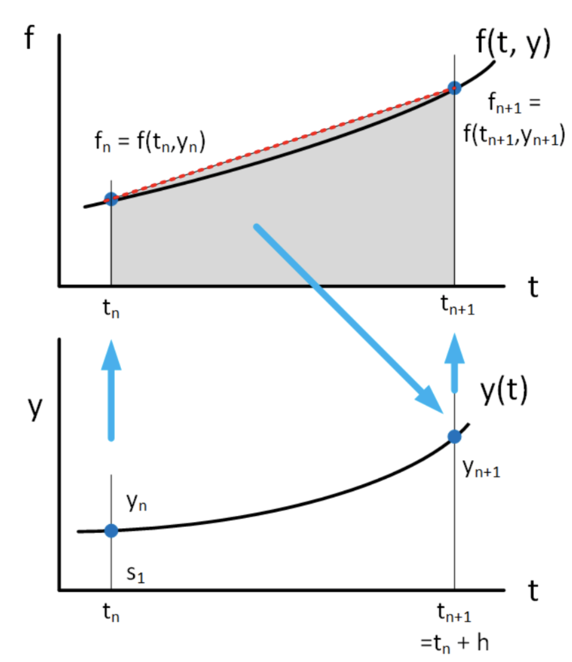
In this case, [eq:6.2] becomes \[\tag{eq:6.4} y_{n+1} = h \int_{0}^{1} \left( (1-\alpha) f_n + \alpha f_{n+1} \right) d \alpha + y_n\] which integrates to \[\tag{eq:6.5} y_{n+1} = \frac{h}{2} \left( f_{n+1} + f_n \right) + y_n\] This is an iteration which takes us from \(t_n\) to \(t_{n+1}\). Here are some things to note about [eq:6.5]:
- This is an implicit method – to get \(y_{n+1}\) on the LHS you need to know \(f_{n+1}\) which depends upon \(y_{n+1}\). Fortunately, we already know how to deal with implicit methods – use a rootfinder like Newton’s method.
- The equation whose root to find is \(g(y_{n+1}) = y_{n+1} -\frac{h}{2} \left( f_{n+1} + f_n \right) - y_n = 0\) where \(f_{n+1} = f(t_{n+1}, y(t_{n+1}))\) and \(f_{n} = f(t_{n}, y(t_{n}))\) as usual.
- This method has approximated \(f(t)\) using a straight line between the two end points, and then integrated the approximation. This is exactly the same as the "trapezoidal method" for numerical integration which you may have seen in a previous numerical analysis class. Therefore, this ODE solver is called the "trapezoidal method".
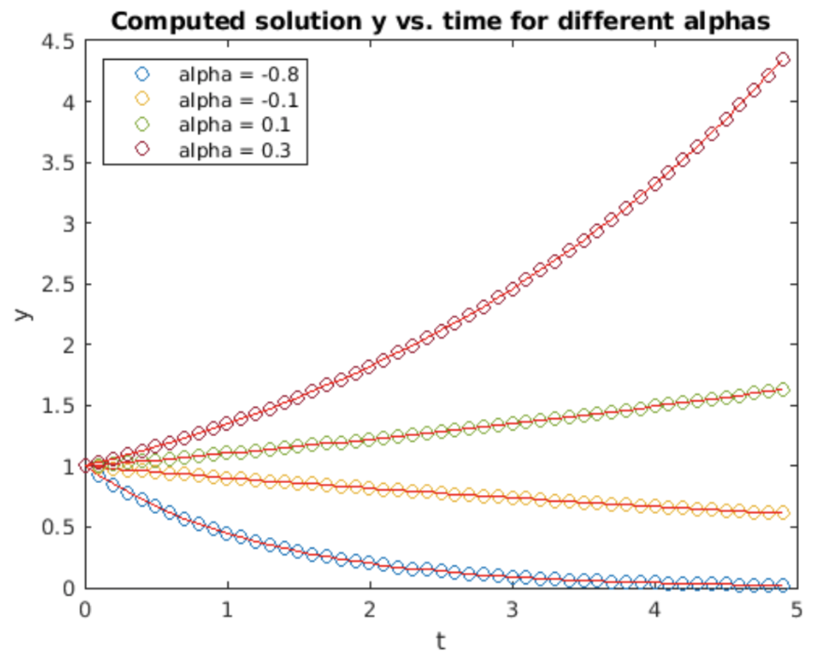
Example: the exponential growth ODE
Adams-Bashforth method – 2nd order
The trapezoidal method uses linear interpolation between points at \(t_n\) and \(t_{n+1}\). It is an implicit method, meaning that it assumes we know the end value \(y_{n+1}\) in order to compute the step using \(f_{n+1} = f(t_{n+1}, y_{n+1})\). However, the step computation is what is used to get the end value \(y_{n+1}\). Therefore, computing the step requires a solve operation to untangle \(y_{n+1}\) from \(f_{n+1}\). A solve operation is generally expensive – solvers like Newton’s method are iterative and one might need several iterations before the solution is found. Wouldn’t it be better to somehow use the linear interpolation to create an explicit method requiring no solver step?
The explicit 2nd order Adams-Bashforth method is such a method. It uses the known (previously computed) values at times \(t_n\) and \(t_{n+1}\) to compute the value at \(t_{n+2}\). The idea is shown in 6.4. In a sense, Adams-Bashforth takes the interpolation formula [eq:6.3] defined on \(t \in [t_n, t_{n+1}]\) and
extrapolates it forward to time \(t_n+2\). That is, it computes the integral
\[\tag{eq:6.6} y_{n+2} = \int_{t_{n+1}}^{t_{n+2}} f_{n, n+1}(t, y(t)) dt + y_{n+1}\] using the approximation to \(f_{n, n+1}\) based on the linear interpolation formula defined on \(t \in [t_n, t_{n+1}]\), [eq:6.3]. We transform the integral [eq:6.6] via the usual change of variables \(\alpha = (t - t_n)/h\) to get \[\tag{eq:6.7} y_{n+2} = h \int_{1}^{2} \left( (1-\alpha) f_n + \alpha f_{n+1} \right) d \alpha + y_{n+1}\] Upon integration we get the second order Adams-Bashforth method,
\[\tag{eq:6.8} y_{n+2} = h \left( \frac{3}{2} f_{n+1} - \frac{1}{2} f_{n} \right) + y_{n+1}\]
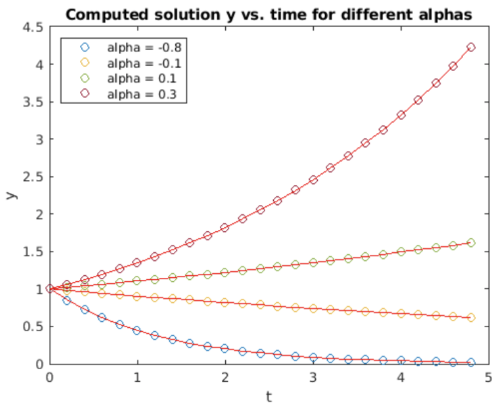
Notice that second-order Adams-Bashforth uses two samples of the function at \(t_n\) and \(t_{n+1}\) to compute the future value at \(t_{n+2}\). This is an explicit method since we presumably already know \(f_{n+1}\) and \(f_n\) when computing \(f_{n+2}\). But this begs the question, how to start this iteration? That is, we have only one initial condition, \(y_0\), but need two \(y\) values to iterate. The answer is that one can start with \(y_0\), then use a single step of e.g. forward Euler or Runge-Kutta to get \(y_1\), then continue the solution using Adams-Bashforth. This is the method employed in the Matlab program whose output is shown in 6.5. Note that the accuracy is \(O(h^2)\), as expected from a second-order method.
Adams-Bashforth method – 3rd order
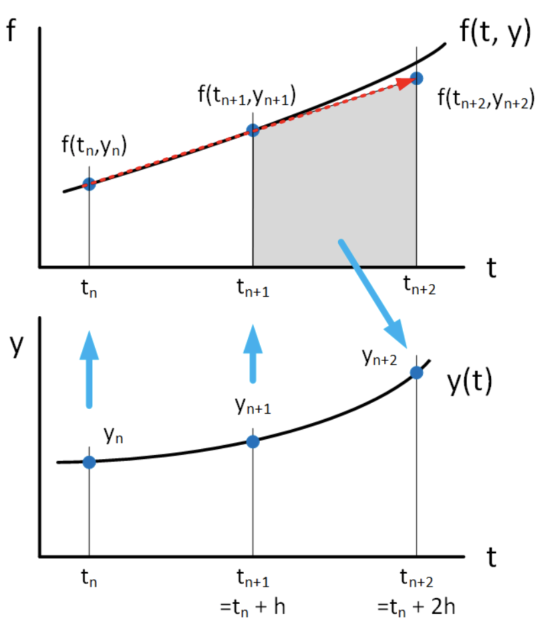
The second-order Adams-Bashforth method used linear interpolation to approximate the function \(f(t,y)\) over the interval \(t_n \le t \le t_{n+1}\), then used that approximation in the integral [eq:6.2] to find \(y_{n+1}\). What if you want more accuracy? Can you use quadratic interpolation on three past points to find the future value? The answer is "yes", and the advantage to this is that the order of the method increases. In this section we will derive the third-order Adams-Bashforth method (quadratic interpolation).
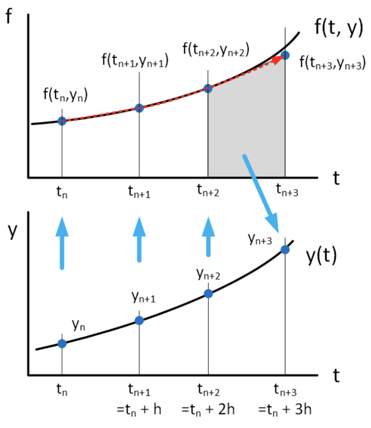
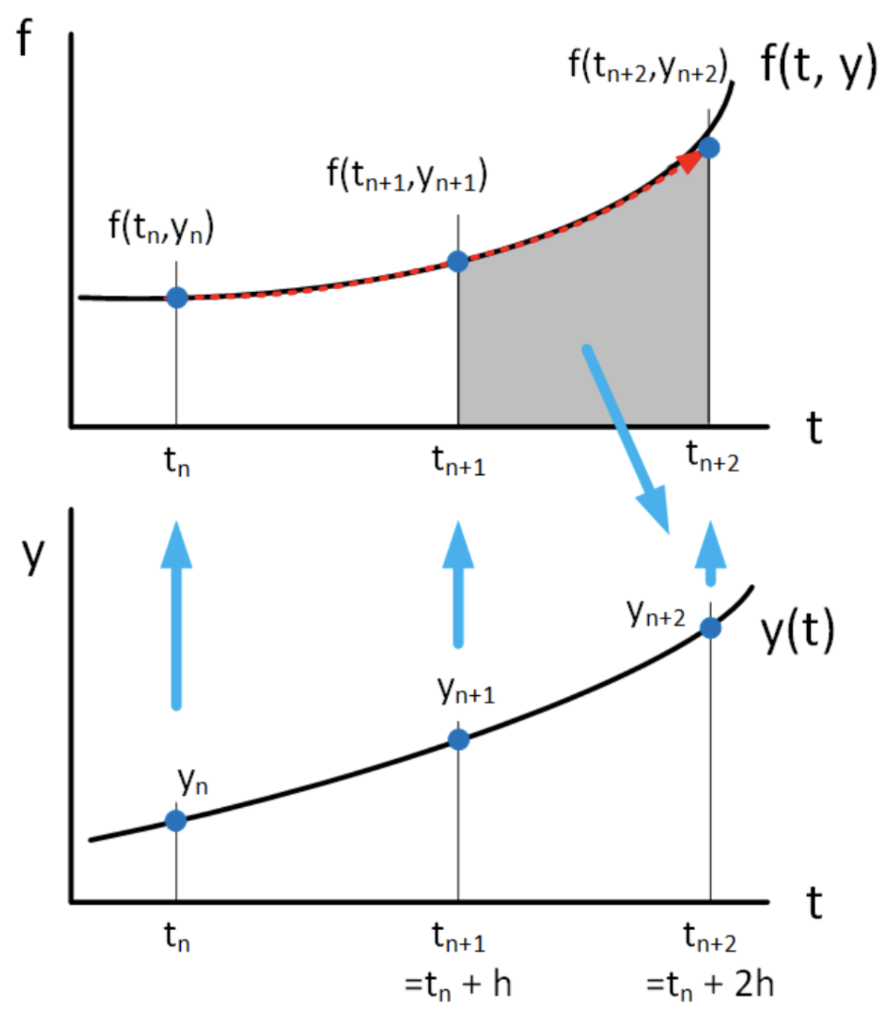
Given two points \((t_n, y_n)\) and \((t_{n+1}, y_{n+1})\) we can draw a straight line through them. Given three points, we can draw a quadratic (a parabola) through them. This is the process of interpolation which you have likely studied in a previous math class. Given a set of points, there are several ways to write down an interpolating polynomial which passes through them. In this case, we are given three points, \((t_n, y_n)\), \((t_{n+1}, y_{n+1})\), and \((t_{n+2}, y_{n+2})\), and we will use the Lagrange interpolation polynomial to write down the quadratic. It is \[\begin{gathered} \label{eq:LagrangeInterpolation} \nonumber f(t) = \frac{(t-t_{n+1})(t-t_{n+2})}{(t_{n}-t_{n+1})(t_{n}-t_{n+2})} f_{n} +\frac{(t-t_{n})(t-t_{n+2})}{(t_{n+1}-t_{n})(t_{n+1}-t_{n+2})} f_{n+1} \\ \nonumber +\frac{(t-t_{n})(t-t_{n+1})}{(t_{n+2}-t_{n})(t_{n+2}-t_{n+1})} f_{n+2}\end{gathered}\] \[\label{eq:LagrangeInterpolation1} \nonumber = \frac{(t-t_{n+1})(t-t_{n+2})}{2 h^2} f_{n} +\frac{(t-t_{n})(t-t_{n+2})}{-h^2} f_{n+1} +\frac{(t-t_{n})(t-t_{n+1})}{2 h^2} f_{n+2}\] This expression might look nasty, but note that it is just a quadratic: Every term is second order in \(t\). Now we insert this expression into the integral [eq:6.2] to find \(y_{n+3}\): \[\nonumber y_{n+3} = \int_{t_{n+2}}^{t_{n+3}} \frac{(t-t_{n+1})(t-t_{n+2})}{2 h^2} f_{n} +\frac{(t-t_{n})(t-t_{n+2})}{-h^2} f_{n+1} +\frac{(t-t_{n})(t-t_{n+1})}{2 h^2} f_{n+2} dt + y_n\] The thing to note is that we use previous points \((t_{n}, y_{n})\), \((t_{n+1}, y_{n+1})\), \((t_{n+2}, y_{n+2})\) to create an approximate version of \(f(t, y)\) using interpolation. Then we integrate that approximation over the interval \(t \in [t_{n+2}, t_{n+3}]\) to get \(y_{n+3}\). The method is shown schematically in 6.7.
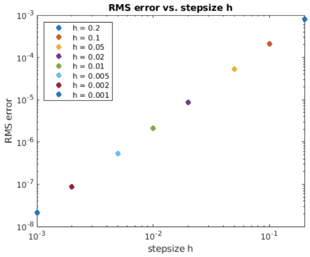
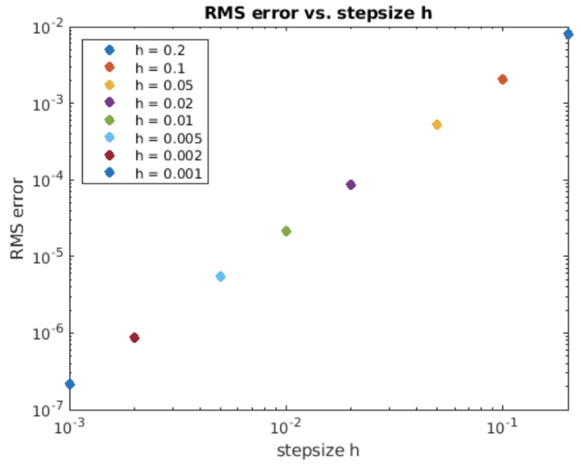
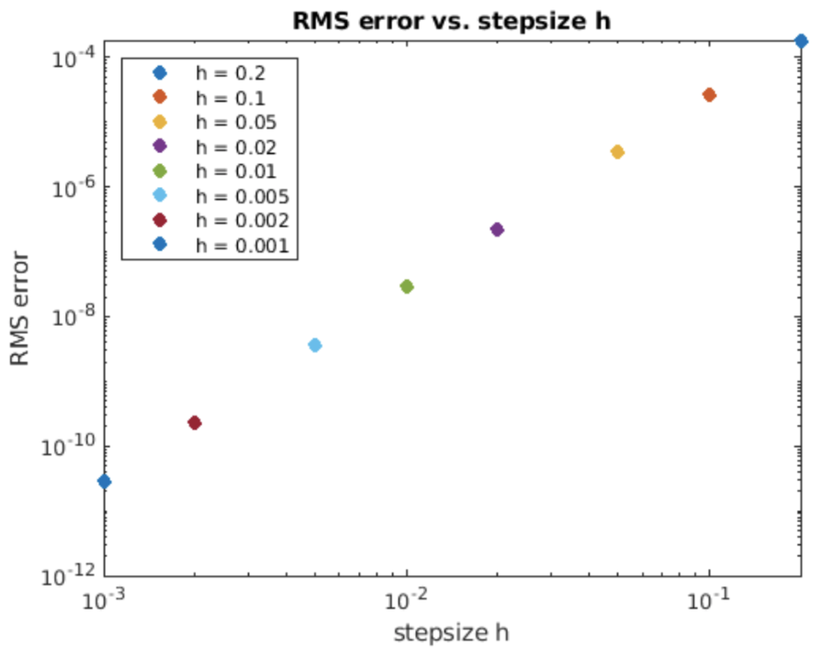
We could carry out the integration immediately, but it would be rather messy. Therefore, we employ the usual change of variables \(\alpha = (t - t_{n+1})/h\). Note that \(h d\alpha = dt\), and that we have mapped \(t = t_{n} \rightarrow \alpha = -1\), \(t = t_{n+1} \rightarrow \alpha = 0\), \(t = t_{n+2} \rightarrow \alpha = 1\), and \(t = t_{n+3} \rightarrow \alpha = 2\). Therefore, the integral becomes \[\nonumber y_{n+3} = h \int_{1}^{2} \frac{1}{2} \alpha(\alpha-1) f_{n} -(\alpha+1)(\alpha-1) f_{n+1} +\frac{1}{2} (\alpha+1)\alpha f_{n+2} d\alpha + y_n\] or \[\tag{eq:6.9} y_{n+3} = h \left( \frac{5}{12} f_{n} -\frac{4}{3} f_{n+1} +\frac{23}{12} f_{n+2} \right) + y_{n+2}\] is the third-order Adams-Bashforth method. As you might expect for a third-order method, the accuracy is order \(O(h^3)\). Plots of its solution to the exponential growth ODE and error scaling are shown in 6.8 and 6.9.
Adams-Moulton method – 3nd order
The Adams-Bashforth methods are explicit – they use the value of \(y\) at the present and past times to compute a the step into the future. Multistep methods may also be implicit – the trapezoidal method is an example of a implicit multistep method you have already see above. Higher order implicit multistep methods also exist. One class are the Adams-Molulton methods. Like Adams-Bashforth, they use interpolation to fit a polynomial to the previous \(f(t,y)\) values, but Adams-Moulton methods incorporate the future \(y\) into the interpolation too. The basic idea is shown in 6.10. The method interpolates the function \(f(t,y)\) at the points \(t_0\) (past), \(t_1\) (present), and \(t_2\) (future) using the Lagrange polynomial \[\begin{gathered} f(t) = \frac{(t-t_{n+1})(t-t_{n+2})}{(t_{n}-t_{n+1})(t_{n}-t_{n+2})} f_{n} +\frac{(t-t_{n})(t-t_{n+2})}{(t_{n+1}-t_{n})(t_{n+1}-t_{n+2})} f_{n+1} \\ \nonumber +\frac{(t-t_{n})(t-t_{n+1})}{(t_{n+2}-t_{n})(t_{n+2}-t_{n+1})} f_{n+2}\end{gathered} \tag{eq: 6.10} \] so the iteration is \[\tag{eq:6.11} y_{n+2} = \int_{t_{n+2}}^{t_{n+3}} \frac{(t-t_{n+1})(t-t_{n+2})}{2 h^2} f_{n} +\frac{(t-t_{n})(t-t_{n+2})}{-h^2} f_{n+1} +\frac{(t-t_{n})(t-t_{n+1})}{2 h^2} f_{n+2} dt + y_{n+1}\] Note that \(f_{n+2} = f(t_{n+2}, y_{n+2})\) so \(y_{n+2}\) appears on both sides of [eq:6.11] – the method is implicit. Nonetheless, we can treat it as a constant factor \(f_{n+2}\) and go ahead and perform the integral. Change variables as usual: \(\alpha = (t-t_0)/h\) so \(h d\alpha = dt\) and the integral becomes \[\tag{eq:6.12} y_{n+2} = h \int_1^2 \frac{(\alpha-1)(\alpha-2)}{2} f_{n} -\alpha(\alpha-2) f_{n+1} +\frac{\alpha(\alpha-1)}{2} f_{n+2} dt + y_{n+1}\]
Evaluating each term yields the third-order Adams-Moulton method: \[\tag{eq:6.13} y_{n+2} = h \left( -\frac{1}{12} f_n + \frac{2}{3} f_{n+1} + \frac{5}{12} f_{n+2} \right) + y_{n+1}\] Again, since \(f_{n+2} = f(t_{n+2}, y_{n+2})\), the equation [eq:6.13] must be solved using a rootfinder to get \(y_{n+2}\), but you should be comfortable with such implicit methods by now.
Example: Adams methods and the Van der Pol oscillator
Here is a quick demonstration showing why implicit methods like Adams-Moulton are useful, despite requiring a rootfinder.
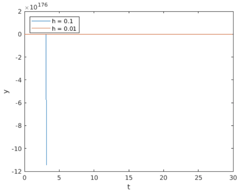
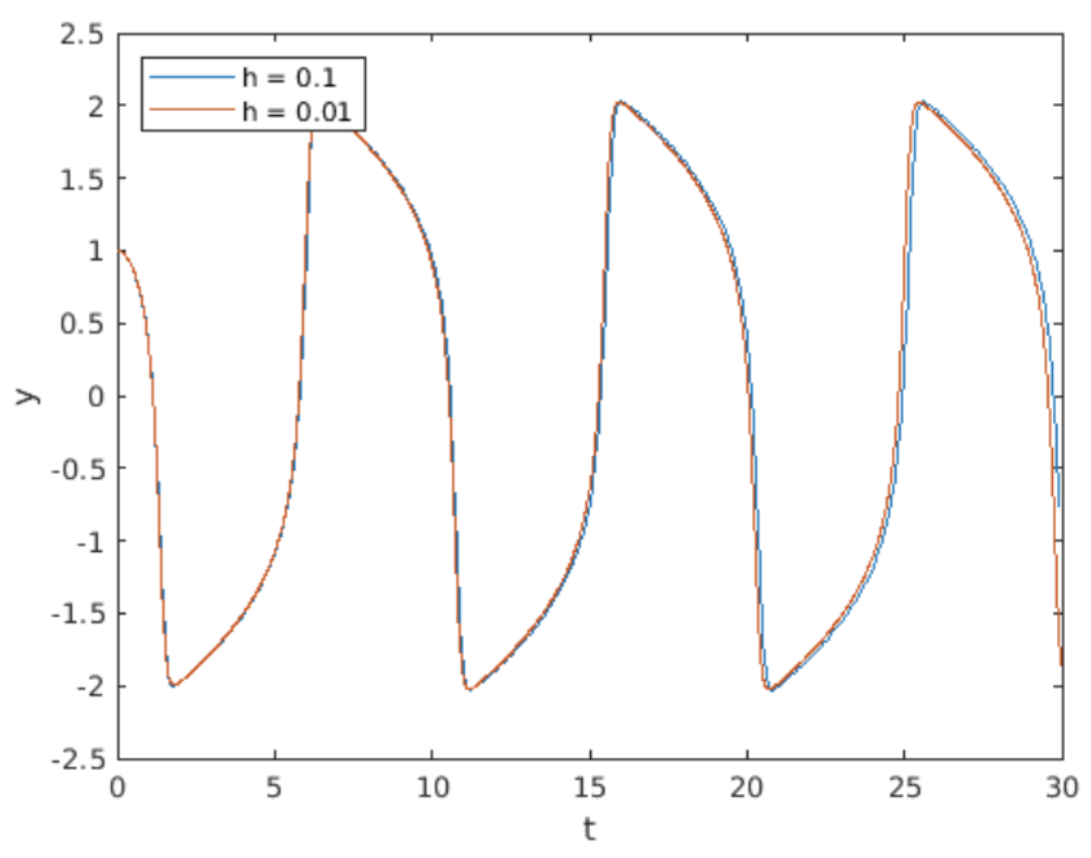
I have written programs implementing 3rd order Adams-Bashforth and 3rd order Adams-Moulton to integrate the Van der Pol oscillator [eq:4.5]. Recall that the Van der Pol system is stiff, and good practice recommends you use implicit methods when integrating stiff ODEs. The reason is that implicit systems can use larger stepsizes without difficulty, so they can quickly solve a stiff system which would force an explicit method like Adams-Bashforth to use small steps.
Shown in 6.11 and 6.12 are plots of the Van der Pol solution computed by 3rd order Adams-Bashforth (explicit) vs. 3rd order Adams-Moulton (implicit). Both solvers used stepsize \(h = 0.1\). At first glance, the result of the Adams-Bashforth computation looks odd. The reason is that the Adams-Bashforth method became unstable, so its output exploded to roughly \(y = -1e177\) – the method is useless for Van der Pol at this stepsize. (Of course, you can decrease the stepsize at the cost of a longer simulation time. That’s not a problem for this toy problem, but if you are faced with a large computation which takes many hours, you want to squeeze as much performance out of your method as possible.) On the other hand, Adams-Moulton works just fine at this stepsize.
I should mention that there is a trade-off between these two methods: Adams-Bashforth requires much smaller stepsize to handle the Van der Pol system, but Adams-Moulton runs a nonlinear solver (Matlab’s fslove()) at each step. Solvers are typically iterative, so they can take significant time to converge on a solution. Therefore, Adams-Bashforth requires less computation per step, but is unstable unless the stepsize is small. On the other hand, the Adams-Moulton method takes longer per step, but remains stable for larger stepsizes. Which method to choose depends upon the particular details of your problem – you typically need to experiment with different methods and different stepsizes to find the best way to solve your particular problem.
Generalizations
There is a whole family of linear multistep methods of orders 2, 3, 4, 5, 6, and so on. The general pattern employed by these methods looks like this: \[\label{eq:LMMGeneralOrder} \alpha_0 y_i + \alpha_1 y_{i+1} + \alpha_2 y_{i+2} + \cdots + y_{i+k} = h \left(\beta_0 f_i + \beta_1 f_{i+1} + \beta_2 f_{i+2} + \cdots + \beta_{k} f_{i+k} \right)\] These are called \(k\)-step methods. Some things to note:
- The coefficient in front of the term \(y_{i+k}\) on the LHS is one. This is the future value which we wish to find.
- If we set all \(\alpha_j = 0\) except \(\alpha_{k-1}\) and additionally set \(\beta_{k}=0\) then we recover the explicit Adams-Bashforth methods.
- If we set all \(\alpha_j = 0\) except \(\alpha_{k-1}\) and keep non-zero \(\beta_{k}\) then we get the Adams-Moulton methods.
- I won’t prove it here, but it can be shown that a \(k\)-step Adams-Bashforth method has order \(O(h^k)\) while a \(k\)-step Adams-Moulton method has order \(O(h^{k+1})\). That’s another advantage of the implicit over the explicit methods.
- Keeping additional \(\alpha_j\) terms gives so-called backward difference methods. Those methods are outside of the scope of this class.
- Regarding stability of linear multistep methods, there is a large body of well-developed theory specifying conditions under which they are stable. That theory is also outside the scope of this class.
High-order linear multistep methods like these are implemented in high-end ODE solvers like the Sundials suite from Lawrence Livermore National Laboratories. Most likely, in your work you will just call such a "canned" solver rather than writing your own, so you are spared the complexities of implementing such a solver.
Chapter summary
Here are the important points made in this chapter:
- Linear multistep methods are derived by interpolating previously-computed (and sometimes future) points and using the interpolation in [eq:6.2] to compute solution points in the future.
- The order of linear multistep methods is increased by incorporating more interpolation points into the interpolated approximation for \(f(t, y)\). We examined the trapezoid (1st order), Adams-Bashforth (2nd and 3rd order), and Adams-Moulton (3rd order) methods.
- Adams-Bashforth methods are explicit, Adams-Moulton are implicit.
- Implicit methods like Adam-Moulton are recommended for stiff systems since they remain stable while also allowing for larger steps than explicit methods. However, implicit methods require running a rootfinder at every step, so a performance trade-off exists between explicit and implicit methods.
- The methods examined in this chapter are members of a large class of linear multistep methods described by [eq:6.14]. Such methods are commonly provided in high-end ODE solvers.