1.5: Adaptive stepping

Choosing \(h\)

Up until now I have not said much about what stepsize \(h\) to choose. Of course, accuracy and stability considerations suggest a smaller stepsize is usually better than a larger one. However, if your stepsize is too small, then your program will take longer to run than necessary to get an accurate answer. There is a trade-off between runtime and stepsize. Runtime doesn’t matter much when running the toy programs used to demonstrate the different methods in this booklet, but if you are doing a gigantic, real-world calculation then you don’t want to waste time if you don’t have to. Oftentimes, the runtime of your program is important – if your program is meant to predict tomorrow’s weather but your program takes 48 hours to run, then your program is useless.

As a first step, if you know something about your ODE, and in particular know the timescale on which you expect to see the solution change, then choosing a stepsize to fit that time scale is easy. However, you commonly don’t know much about your solution’s behavior, which is why you are simulating it in the first place. Also, your ODE might behave badly – the solution might be smooth and slowly-varying for one period of time, then become bursty or quickly-varying at a subsequent time. Because of this, adaptive stepping is a common method useful to find the best stepsize for your simulation. The idea is simple:

1. Take a single step of size \(h\).
2. Estimate the error between the true solution and your step.
3. If the error is too large, then go back and retry your step with a smaller stepsize, for example \(h/2\). Then use this step size moving forward.
4. However, if the error is small enough, increase the stepsize for future steps.
5. Go back to 1 and continue stepping.

The idea is that the error incurred at each step can stay below some bound. In rough terms, if your solution changes slowly then you may take larger steps. But if your solution changes quickly, then you need to take smaller steps in order to maintain good accuracy.

Of course, the big question is, how to estimate the error? In the best case you could compare your computed solution against the true solution – but if you already had the true solution then you wouldn’t need to run an ODE solver in the first place! As a second-best case, you could use a so-called "oracle". In computer science, an oracle is a function or a program you can ask if your solution is true or not. That is, you can compute a step, then give the result to an oracle and it will say either "yes, your solution is correct" or "no, your solution is wrong". As a thought-experiment the oracle is generally regarded as a "black box", meaning that you don’t necessarily know how it works on the inside. It’s enough to simply know that the oracle will either say "yes" or "no" to your proposed answer, and the oracle will give an accurate judgement.

What is a good oracle for use with an ODE solver? Here are two possibilities:

1. A simple idea is to just run each step twice: first use stepsize \(h\), then take two steps of stepsize \(h/2\) and compare the results. In this case, the \(h/2\) steps may be regarded as a sort of oracle since its answer is (presumably) more accurate than the \(h\) step. The problem with this scheme is that you effectively run the solver twice – two times for each step. This makes your program run (at least) twice as long as necessary.
2. You could also consider taking a step using, say, forward Euler, and then taking the same step using, say, Heun’s method. The idea here is that since forward Euler is \(O(h)\) but Heun’s method is \(O(h^2)\) then Heun’s method is a good oracle. Again, this means you waste significant time recomputing your step. On the other hand, in Heun’s method you can reuse the initial forward Euler step, so you get back some some performance through reuse of previously computed results.

It turns out that real-world solvers use a variant of possibility 2. Recall the fourth-order Runge-Kutta method from 4.6. The RK4 method presented there is a member of a larger family of Runge-Kutta methods of varying order. Matlab’s famous ode45() solver uses a method called Dormand-Prince order 4/5. In this solver, two Runge-Kutta methods are used. The first is a 4th-order Runge-Kutta variant (not the one presented in 4.6), and the second is a 5th-order Runge-Kutta method. The coefficients used to compute the intermediate steps of both methods are the same, only the final computation is different. Therefore, the amount of additional computation required to implement the oracle check is a small part of the overall calculation at each step. The combined Butcher tableau of the methods used in ode45() are shown in [tab:5.1]. You can also see these parameters in Matlab by issuing the command "dbtype 201:213 ode45", which emits the Butcher table in a slightly different form than above.

Regarding changing the step size, my naive suggestion in item 1 either halves or doubles the step size depending upon the error measured by the method. A better approach would be to tune the step size depending upon the magnitude of the observed error. That is, make the new step size depend upon the actual error observed instead of blindly halving or doubling the step. Algorithms for doing such fine-tuning exist, but are outside the scope of this booklet.

Table 5.1: Butcher tableau for the Dormand-Prince 4/5 solver used in Matlab’s ode45(). The two rows below the horizontal line correspond to the two corrector steps which are compared against each other.

0	0	0	0	0	0	0	0
1/5	1/5	0	0	0	0	0	0
3/10	3/40	9/40	0	0	0	0	0
4/5	44/45	-56/15	32/9	0	0	0	0
8/9	19372/6561	-25360/2187	64448/6561	-212/729	0	0	0
1	9017/3168	-355/33	46732/5247	49/176	-5103/18656	0	0
1	35/384	0	500/1113	125/192	-2187/6784	11/84	0
	35/384	0	500/1113	125/192	-2187/6784	11/84	0
	5179/57600	0	7571/16695	393/640	-92097/339200	187/2100	1/40

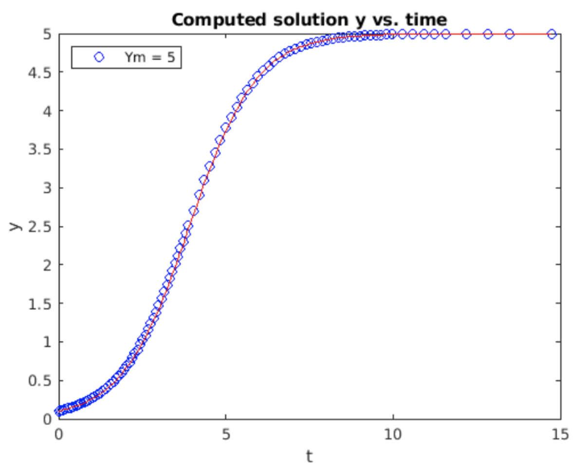
Example: the logistic equation

Instead of demonstrating the full Dormand-Prince 4/5, I will show a simpler adaptive stepper based on possibility 2 above. The program algorithm is shown in [alg:6]. I use the logistic equation as the example because the solution has (roughly) two regions of interest: A quickly varying phase of exponential growth at the beginning of the run followed by a plateau as \(t \rightarrow \infty\). Results obtained from the Matlab implementation of the program are shown in 5.1. The step size clearly remain small during the beginning of the run, but when the solution stabilizes (doesn’t change) the step size increases. This is particularly evident for times \(t > 10\).

__________________________________________________________________________________________________________________________________

Algorithm 6 Naive adaptive step method

__________________________________________________________________________________________________________________________________

Inputs: initial condition \(y_0 = [u_0, v_0]^T\), end time \(t_{end}\).

Initialize: \(t_0 = 0, y_0, h\).

Initialize: \(tol_1 = 1e - 2, tol_2 = 2e-4\).

for \(n=0: t_{end}/h\) do

Get inital slope: \(s_1 = f(t_n, y_n)\)

Take forward Euler step: \(y_{fe} = y_n + h s_1\)

Get slope at new position: \(s_2 = f(t_n, y_{fe})\)

Take Heun step: \(y_h = y_n + h (s_1+s_2)/2\)

Check difference between Euler and Heun steps: \(\delta = ||y_{fe}-y_h||\)

if \(\delta > tol_1\) then

Error too large - decrease step: \(h=h/2\)

else if \(\delta < tol_2\) then

Error very small - increase step: \(h=2h\)

else

Error neither too small or too large. Keep step.

end if

end for

return \(y_n\).

Figure 5.1: Example run of my naive adaptive step solver on the logistic ODE. This solver computes a forward Euler step, then computes a Heun’s method step to use as the oracle. When the results of the two steps disagree, the solver halves the stepsize and tries again. When the steps agree closely, the solver doubles the stepsize for the next step. Otherwise the solver continues iterating using the current step. The step size increases for slowly-varying portions of the solution are evident at times \(t > 10\). The red line is the analytic solution.

Stiff ODEs

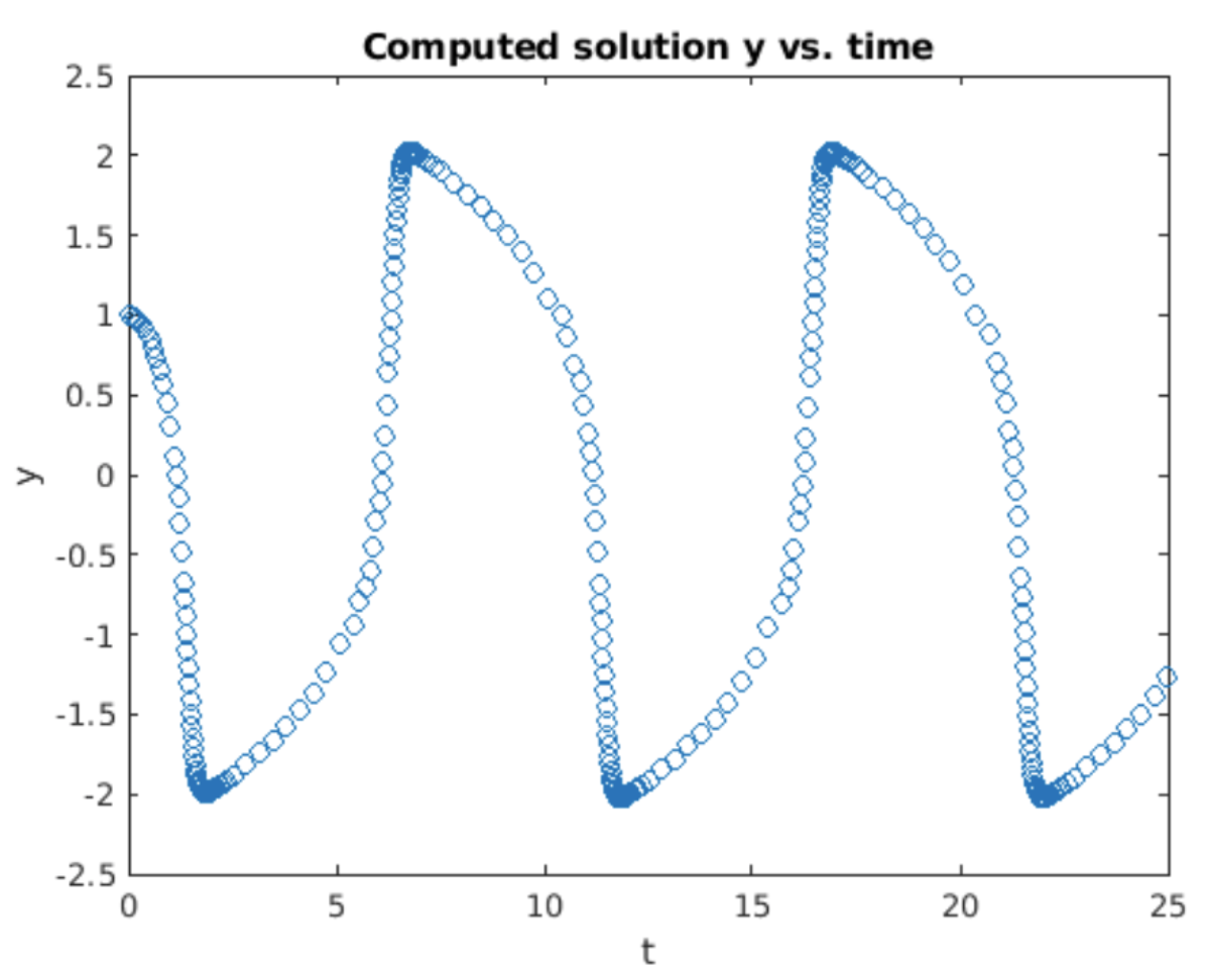
In the last section we saw an adaptive step method which took small steps when the solution varied quickly, and took larger steps when the solution varied slowly. The concept of slow vs. fast varying generalizes to the concept of "stiffness" of an ODE. An exact definition of the term "stiff" is hard to pin down, but the basic intuition is that a stiff ODE is one where you need to take small steps at some times to maintain accuracy, but can take much larger steps at other times. The problem with a stiff ODE is that if you use a fixed time step \(h\), then you need \(h\) to be very small for those sections of the ODE requiring small steps. However, stepping then proceeds slowly over sections where you could use a large \(h\) and step quickly – meaning you are wasting compute time! Dealing with stiffness is why adaptive solvers are so important.

The Van der Pol equation is a common example of a stiff ODE. The solution computed using the adaptive stepper is shown in 5.2. When the solution peaks out at around \(y \approx \pm 2\) the step size must decrease significantly to maintain an accurate solution. Inspecting the phase plot 5.3 shows another view of this phenomenon – when the solution takes a hard right turn the step size must decrease to follow the solution, but the step size may increase when the solution moves away from the "right turn". The question is, why does the step size need to decrease at these points

Figure 5.2: The Van der Pol equation integrated using my naive adaptive step solver. Note that the solver takes small steps at the "corners" where the solution saturates at a value \(y \approx \pm 2\).

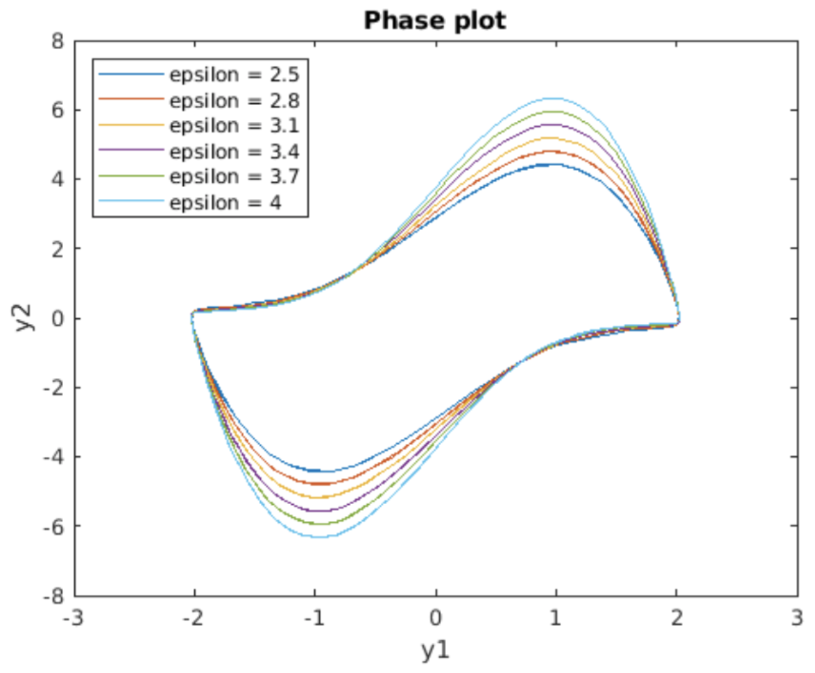
in the phase plane, but not in others? The answer comes from considering the entire family of solutions to the Van der Pol equation in the phase plane. A plot of the situation is shown in 5.4, which is a phase plot for varying values of \(\epsilon\). The solutions for varying \(\epsilon\) are bunched together at the corners, but spread out away from those regions. Near the corners staying on the correct solution (i.e. not jumping to another solution in the family) depends very sensitively upon closely following the correct solution trajectory. The adaptive stepper somehow "feels" this sensitivity and

Figure 5.3: The phase plot shows that the stepsizes decrease where the solution takes a hard right turn, but increase when the solution moves away from the "corners".

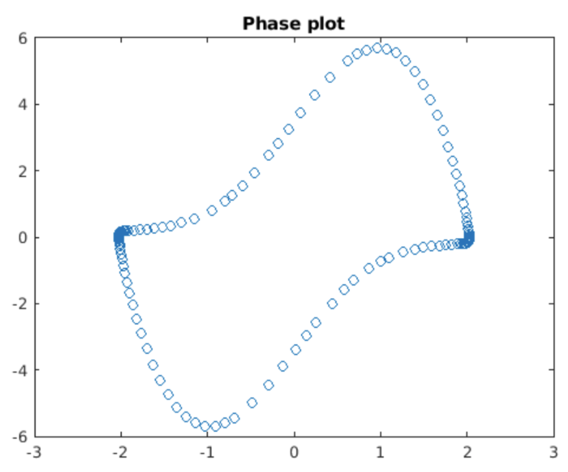
accordingly adjusts the step size to remain on the correct trajectory. The importance of adaptive step size solvers is simply that if the solver did not change its step size, then to get an accurate solution you would need to use a very small step \(h\) to remain on the correct trajectory in the sensitive regions. The sensitive regions are those where the family of solutions lies close to one another. However, small \(h\) means the solver’s run time would be much longer than needed since it would also take small steps through the region where the solution trajectory is relatively insensitive. The adaptive solver is the best of both cases: Fast stepping through the insensitive regions and slow, careful stepping through the sensitive regions.

Figure 5.4: Phase plots for varying values of \(\epsilon\). Note that the solutions are bunched together in the vicinity of the "corners". This signals that finding the correct solution from all solutions in the family depends very sensitively upon the details of the solution trajectory. Small perturbations cause potentially large changes in the trajectory. The adaptive stepper somehow "feels" this sensitivity and accordingly adjusts the step size to remain on the correct trajectory.

Chapter summary

Here are the important points made in this chapter:

• An adaptive step size method changes the step size \(h\) to maintain the solution error remains below some tolerance. When the stepper senses the solution error is growing, it will decrease the step size until the error resulting from a step remains below the tolerance. When the stepper senses that the solution error is small enough, it will increase the step size to speed up the solution.
• A stiff system is one in which the solution evidences regions of fast and regions of slow variation, or more exactly high or low sensitivity to adjacent solutions to the ODE.