1.3: Backward Euler method

Backward Euler algorithm

The next ODE solver is called the "backward Euler method" for reasons which will quickly become obvious. Start with the first order ODE, \[\tag{eq:3.1} \frac{d y}{d t} = f(t, y)\] then recall the backward difference approximation, \[\nonumber \frac{d y}{d t} \approx \frac{y_n - y_{n-1}}{h}\] We can use this in [eq:3.1] to get \[\tag{eq:3.2} \frac{y_n - y_{n-1}}{h} = f(t_n, y_n)\] Since we’re using backward differencing to derive [eq:3.2], this is the "backward Euler method". Now shift this forward in time by one step (i.e. replace \(n\) by \(n+1\) everywhere). This shift creates a valid equation since [eq:3.2] is valid for all \(n\). Upon shifting we get \[\nonumber \frac{y_{n+1} - y_{n}}{h} = f(t_{n+1}, y_{n+1})\] Now move the future to the LHS and the present to the RHS to get \[\tag{eq:3.3} y_{n+1} - h f(t_{n+1}, y_{n+1}) = y_{n}\] Now you might rightly ask, what good does this expression do? In order to compute the unknown \(y_{n+1}\), you need to already know \(y_{n+1}\) to use it on the LHS. But how can you use \(y_{n+1}\) if it’s the unknown you are solving for?

The answer is that you can turn [eq:3.3] into a rootfinding problem. Subtract the known value \(y_n\) from both sides of [eq:3.3]. Then consider the expression on the LHS to be a function of \(y_{n+1}\). We have \[\tag{eq:3.4} g(y_{n+1}) = y_{n+1} - h f(t_{n+1}, y_{n+1}) - y_{n} = 0\] Therefore, finding \(y_{n+1}\) involves finding the root of \(g(y_{n+1})\). In general, \(g(y_{n+1})\) can be a nasty, non-linear function of \(y_{n+1}\), but such problems are easily handed using numerical methods – Newton’s method immediately springs to mind. We won’t cover rootfinding in this class, but many methods are presented in the standard texts on numerical analysis.

Assuming you can use a rootfinding method to solve [eq:3.4], you have a time-stepping method: Start with the initial condition \(y_0\), insert it into [eq:3.4], then use rootfinding to compute \(y_1\). Then using \(y_1\) use [eq:3.4] and rootfinding to find \(y_2\), and so on. This is the backward Euler method.

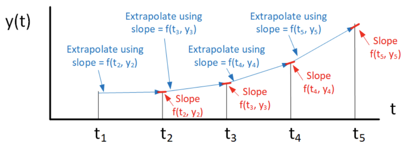
Pseudocode implementing the backward Euler algorithm to solve the simple harmonic oscillator is shown in [alg:3]. A graphical depiction of the algorithm is shown in fig. 3.1. 

__________________________________________________________________________________________________________________________________

Algorithm 3 Backward Euler method

__________________________________________________________________________________________________________________________________

Inputs: initial condition \(y_0\), end time \(t_{end}\).

Initialize: \(t_0 = 0, y_0\).

for \(n = 0: t_{end}/h\) do

Form equation for LHS with \(y_{n+1}\) as unknown variable, \(g(y_{n+1}) = y_{n+1} - h f(t_{n+1}, y_{n+1}) - y_{n}\)

Solve rootfinding problem \(g(y_{n+1}) = 0\) to find \(y_{n+1}\).

end for 

return \(y\) vector.

__________________________________________________________________________________________________________________________________

Figure 3.1: The backward Euler algorithm. At each time step the algorithm uses rootfinding to get the slope of \(y\), then moves forward by step \(h\). The slope used is that at the end of the interval.

Here are some things to note about backward Euler:

• Note that the slope used is the slope at the end of the step interval – hence the name "backward" Euler. You can see how each step is determined by the slope of the blue line.
• The step is not directly calculable from the RHS of [eq:3.3]. Rather, rootfinding is required to get the value of \(y_{n+1}\) at each step. Therefore, backward Euler is called an "implicit method".

Example: exponential growth ODE

As an example of backward Euler we again consider the exponential growth ODE, \[\tag{eq:3.5} \frac{d y}{d t} = \alpha y\] Discretize using the backward difference approximation to get \[\nonumber \frac{y_{n+1} - y_n}{h} = \alpha y_{n+1}\] Move the future to the LHS and the present to the RHS to get \[\nonumber y_{n+1} - h \alpha y_{n+1} = y_n\] Since this is a linear equation, deriving the time-stepping method is easy – no rootfinding required. 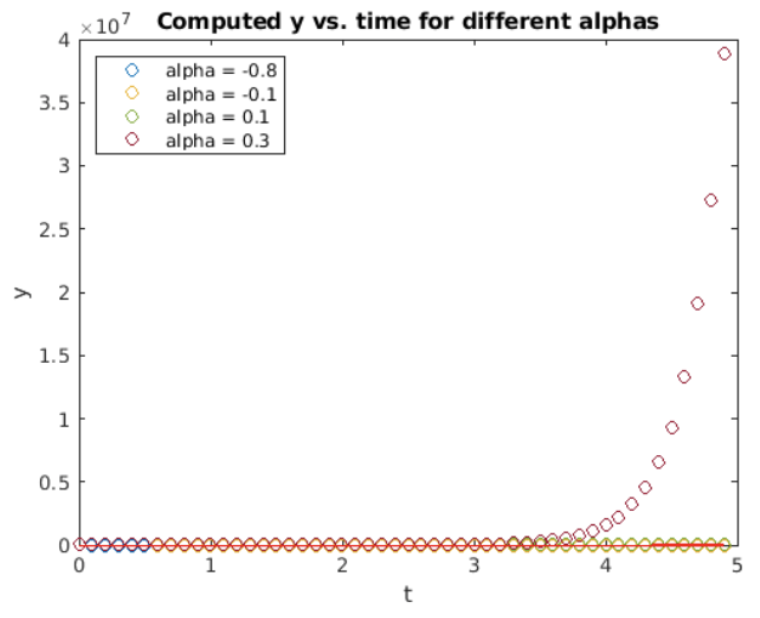We obtain \[\tag{eq:3.6} y_{n+1}= \frac{y_n}{1 - h \alpha }\] A plot of the solution found via backward Euler when \(h = 0.1\) is shown in fig. 3.2. Something is wrong! The plots do not look like those shown in fig. 2.3, nor do they match the analytic result. What happened?

Figure 3.2: Backward Euler solution of the exponential growth ODE for \(h = 0.1\). Something is obviously wrong!

The biggest hint is the y-axis scale – it says one of the curves increases to around 4e7 – a gigantic number. This is a clear signal backward Euler is unstable for this system. Stability is therefore the subject of the next subsection.

Stability of backward Euler for the exponential growth ODE

Now we derive the domain of stability for the backward Euler method. We again consider the exponential growth equation [eq:3.5] first presented in section 2.2. Following an argument similar to that presented in section 2.2 we may derive the following expression for the growth of an initial perturbation: \[\nonumber e_{n+1} = \frac{e_n}{1 + a h}\] Note the similarity of this expression to [eq:3.6] in the last section. The similarity holds because of the linearity of [eq:3.5]. 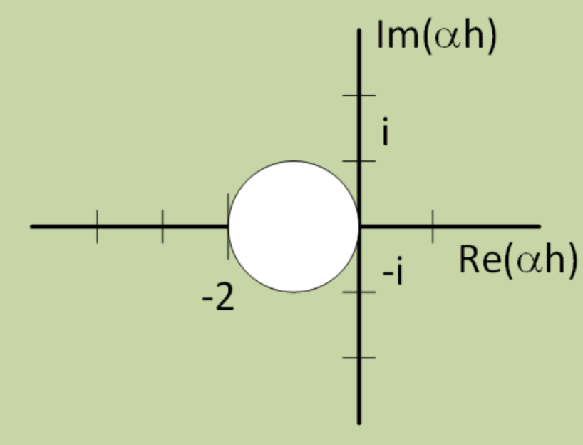Assuming the start perturbation at time \(t=0\) is \(e_0\), the error grows as \[\tag{eq:3.7} e_n = \left( \frac{1}{1+a h} \right)^n e_0\] For the error to remain bounded, we require \[\nonumber \left| \frac{1}{1+a h} \right| \le 1\] or \[\tag{eq:3.8} \left| 1+a h \right| \ge 1\] A plot of the region in the complex plan where the error is bounded (i.e. where backward Euler is stable for this ODE) is shown in fig. 3.3. Note that this stability region is the complement of that obtained for forward Euler – backward Euler is stable for large relative step values (large \(a h\)) while forward Euler is only stable for small steps. Compare the stability regions shown here to that shown in fig. 2.10.

Figure 3.3: Backward Euler’s stability region for the exponential growth ODE [eq:3.5]. The stability region includes the entire complex plane with the exception of the circle of radius 1 in the complex plane centered at \(a h = -1\).

Thinking back to the results obtained in section 3.2 for the exponential growth ODE, recall we set \(h = 0.1\) and simulated a number of different \(\alpha\) values. For each \(\alpha\) value we have

• \(\alpha = -0.8\), \(\alpha h = -0.08\). This lies inside the unstable circle in 3.3. Unstable!
• \(\alpha = -0.1\), \(\alpha h = -0.01\). This lies inside the unstable circle in 3.3. Unstable!
• \(\alpha = 0.1\), \(\alpha h = 0.01\). This lies outside the unstable circle in 3.3. Stable.
• \(\alpha = 0.3\), \(\alpha h = 0.03\). This lies outside the unstable circle in 3.3. Stable.

Therefore, the bad results shown in 3.2 are due to the fact that two of the \(\alpha h\) values are in the unstable area.

Example: the logistic equation

Recall the logistic equation, [eq:2.11]. We discretize for backward Euler by putting the future on the LHS and the present on the RHS. In this case the iteration is \[\nonumber y_{n+1} - h \left( 1 - \frac{y_{n+1}}{Y_m} \right)y_{n+1} = y_n\] This is a nonlinear equation, so a rootfinder is required to implement the backward Euler iteration. That is, upon every iteration the following equation is solved to find the value of \(y_{n+1}\) \[\nonumber g(y_{n+1}) = y_{n+1} - h \left( 1 - \frac{y_{n+1}}{Y_m} \right)y_{n+1} - y_n = 0\] The parameters \(h\) and \(Y_m\) are inputs to the problem and are therefore known quantities. Also, since at each step we start at \(t_n\), the value \(y_n\) is also known. That means \(y_{n+1}\) is the only unknown and it is the quantity we solve for. A solver like Newton’s method, or the Matlab built-in function "fsolve()" are perfectly suited to compute the required value of \(y_{n+1}\).

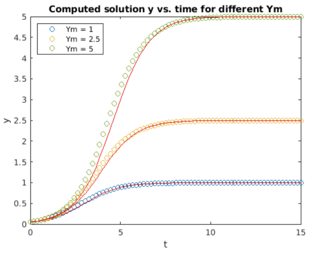
This iteration was implemented in Matlab and then run for three different values of \(Y_m\). The results are shown in 3.4. The computed solution leads the analytic solution. Compare this to 2.6, where the computed solution trails the analytic solution.

Figure 3.4: The solution to the logistic equation [eq:2.11] computed using the backward Euler algorithm for three different \(Y_m\) values. Matlab’s fsolve() was used to compute \(y_{n+1}\) at each step of the method. Note that the computed solution leads (is in front of) the analytic solution. Compare these results to those for the forward Euler iteration in 2.6

Example: the simple harmonic oscillator

To apply the backward Euler method to the simple harmonic oscillator we start with the pair of first order ODEs, \[\begin{aligned} \nonumber \frac{d u}{d t} &= -\frac{k}{m} v \\ \nonumber \frac{d v}{d t} &= u\end{aligned}\] then discretize using the backward difference approximation. We get \[\tag{eq:3.9} \begin{aligned} \frac{u_{n+1} - u_{n}}{h} &= -\frac{k}{m} v_{n+1} \\ \frac{v_{n+1} - v_{n}}{h} &= u_{n+1} \end{aligned}\] Rearranging and moving the future to the LHS and the present to the RHS this becomes \[\begin{aligned} \nonumber u_{n+1} + h \frac{k}{m} v_{n+1} = u_{n} \\ \nonumber v_{n+1} - h u_{n+1}= v_{n} \end{aligned}\] Now we can gather the coefficients on the LHS into a matrix and write this as \[\begin{aligned} \nonumber \begin{pmatrix} 1 & h k / m \\ -h & 1 \end{pmatrix} \begin{pmatrix} u_{n+1} \\ v_{n+1} \end{pmatrix} = \begin{pmatrix} u_{n} \\ v_{n} \end{pmatrix}\end{aligned}\] As with forward Euler, we note that the system [eq:3.9] may be replaced with matrix-vector multiplication because the original equation is linear. If the original system was nonlinear, then you would need to solve it as a system (i.e. you would not be able to simplify it into a matrix-vector multiplication form.)

We want to isolate the future on the LHS and use the RHS to compute the future using known quantities. Therefore, we move the matrix to the RHS to get the iteration, \[\begin{aligned} \begin{pmatrix} u_{n+1} \\ v_{n+1} \end{pmatrix} = \begin{pmatrix} 1 & h k / m \\ -h & 1 \end{pmatrix}^{-1} \begin{pmatrix} u_{n} \\ v_{n} \end{pmatrix}\end{aligned} \tag{eq:3.10}\] Now we have isolated all the known quantities onto the RHS so we have a time-stepping method. In the Matlab implementation we could use the analytic inverse of the \(2 \times 2\) matrix, but instead we will just leave it as it stands and let Matlab perform the computation using a linear solve operation. This is in the spirit of backward Euler, where each step of the algorithm involves inverting the function [eq:3.4] appearing on the LHS. In this case, the function is matrix-vector multiplication, so we just need to invert the matrix (i.e. do a linear solve) to move it to the RHS.

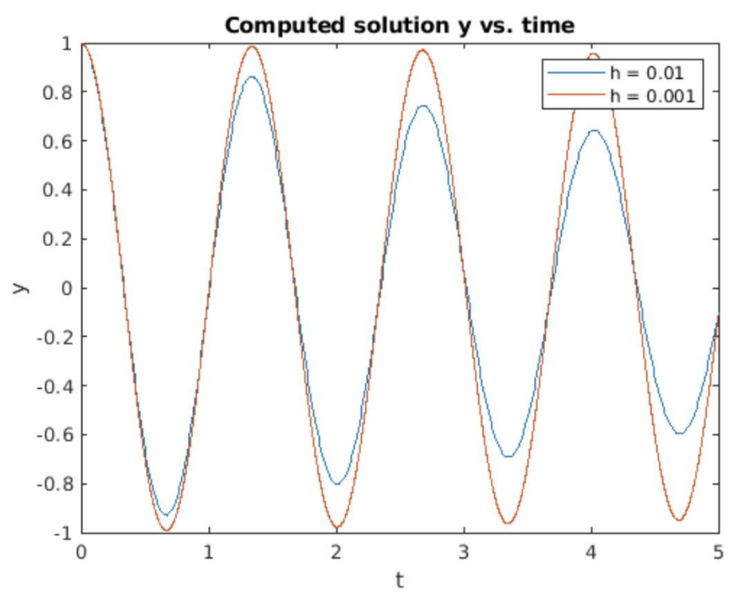
Running the backward Euler SHO algorithm produces the the plot shown in 3.5. In this case we find the sinusoidal oscillations decay with time. For smaller step \(h\) the decay is slower than for larger \(h\). Again, this behavior is not consistent with the analytic solution, which is a sine wave having constant amplitude – that is, no increase nor decay with time.

Figure 3.5: The simple harmonic oscillator solved using backward Euler and a propagator matrix. In contrast to the known mathematically-exact solution, the numerical solution decays exponentially in time. The decay rate is faster for larger step sizes \(h\).

Stability of backward Euler for the simple harmonic oscillator

Understanding why the solution decays involves finding the eigenvalues of the propagator matrix. That is, we will undertake a stability analysis for backward Euler similar to that presented in 2.9.2 for forward Euler. To make life easy we’ll first define \[\tag{eq:3.11} \omega^2 = \frac{k}{m}\] This just makes the algebra easier later. Next, we invert the matrix on the RHS of [eq:3.10]. This gives us the propagator matrix \[\nonumber \begin{pmatrix} \frac{1}{h^2 \omega^2 + 1} & - \frac{h \omega^2}{h^2 \omega^2 + 1} \\ \frac{h}{h^2 \omega^2 + 1} & \frac{1}{h^2 \omega^2 + 1} \end{pmatrix}\] To understand the stability of the iteration we must examine the eigenvalues of the propagator matrix [eq:3.11]. Call the eigenvalues \(g\) for "growth factor". The eigenvalues of this matrix are found by solving \[\nonumber det \begin{pmatrix} \frac{1}{h^2 \omega^2 + 1} - g & - \frac{h \omega^2}{h^2 \omega^2 + 1} \\ \frac{h}{h^2 \omega^2 + 1} & \frac{1}{h^2 \omega^2 + 1} -g \end{pmatrix} =0\] for \(g\). We have \[\nonumber \left(\frac{1}{h^2 \omega^2 + 1} - g \right)^2 + \frac{h^2 \omega^2}{(h^2 \omega^2 + 1)^2} = 0\] so \[\nonumber g = \frac{1 \pm i h \omega}{h^2 \omega^2 + 1}\] or \[\tag{eq:3.12} g = \frac{1}{1 \pm i h \omega}\] Now consider the magnitude (absolute value) of \(g\). The numerator of [eq:3.12] is one while the denominator always has absolute value less than one. Therefore, \(|g| < 1\) always unless \(h=0\) or \(\omega=0\). \(h=0\) is not a useful value since it implies no stepping. Therefore, for any reasonable value of \(h \omega\) the solution obtained by backward Euler will always decrease for any non-zero stepsize \(h\), as is observed in 3.5.

Chapter summary

Here are the important points made in this chapter:

• The backward Euler method is derived from the simple backward difference expression for the derivative, \(y' = (y_{n} - y_{n-1})/h\).
• The backward Euler method is an iterative method which starts at an initial point and walks the solution forward using the iteration \(y_{n+1} - h f(t_{n+1}, y_{n+1}) = y_{n}\).
• Since the future \(y_{n+1}\) appears as a function which must be inverted on the LHS, backward Euler is an implicit method.
• Like any implicit method, a rootfinder – such as Newton’s method – is required to find \(y_{n+1}\) at each step in time.
• The RMS error expected when using the backward Euler method scales as \(e \sim O(h)\).
• Solver stability is not guaranteed for all step sizes \(h\). The stability criterion depends upon the exact ODE under consideration, but forward Euler can be stable for larger step sizes than forward Euler.