3.3.1: Examples

Example 3.3.1.1: Beltrami Equations

$$\begin{eqnarray} \label{belt1}\tag{3.3.1.1} Wu_x-bv_x-cv_y&=&0\\ \label{belt2}\tag{3.3.1.2} Wu_y+av_x+bv_y&=&0, \end{eqnarray}$$

where $W,\ a,\ b,\ c$ are given functions depending of $(x,y)$, $W\not=0$ and the matrix

$$
\left( $$\begin{array}{cc} a&b\\ b&c \end{array}$$ \right)
\]

is positive definite.

The Beltrami system is a generalization of Cauchy-Riemann equations. The function $f(z)=u(x,y)+iv(x,y)$, where $z=x+iy$, is called a quasiconform mapping, see for example [9], Chapter 12, for an application to partial differential equations.

Set

$$
A^1=\left( $$\begin{array}{cc} W&-b\\ 0&a \end{array}$$ \right),\ \
A^2=\left( $$\begin{array}{cc} 0&-c\\ W&b \end{array}$$ \right).
\]

Then the system ($\ref{belt1}$), ($\ref{belt2}$) can be written as

$$
A^1\left( $$\begin{array}{c} u_x\\v_x \end{array}$$ \right)+
A^2\left( $$\begin{array}{c} u_y\\v_y \end{array}$$ \right)=\left( $$\begin{array}{c}0\\0\end{array}$$ \right).
\]

Thus,

$$\begin{eqnarray*} C(x,y,\zeta)=\left|\begin{array}{cc} W\zeta_1&-b\zeta_1-c\zeta_2\\ W\zeta_2&a\zeta_1+b\zeta_2 \end{array}\right| =W(a\zeta_1^2+2b\zeta_1\zeta_2+c\zeta_2^2), \end{eqnarray*}$$

which is different from zero if $\zeta\not=0$ according to the above assumptions. Thus the Beltrami system is elliptic.

Example 3.3.1.2: Maxwell Equations

The Maxwell equations in the isotropic case are

$$\begin{eqnarray} \label{max1}\tag{3.3.1.3} c\ \text{rot}_x\ H&=&\lambda E+\epsilon E_t\\ \label{max2}\tag{3.3.1.4} c\ \text{rot}_x\ E&=&-\mu H_t, \end{eqnarray}$$

where

• $E=(e_1,e_2,e_3)^T$ electric field strength, $e_i=e_i(x,t)$, $x=(x_1,x_2,x_3)$,
• $H=(h_1,h_2,h_3)^T$ magnetic field strength, $h_i=h_i(x,t)$,
• $c$ speed of light,
• $\lambda$ specific conductivity,
• $\epsilon$ dielectricity constant,
• $\mu$ magnetic permeability.

Here $c,\ \lambda,\ \epsilon$ and $\mu$ are positive constants.

Set $p_0=\chi_t,\ p_i=\chi_{x_i}$, $i=1,\ldots 3$, then the characteristic differential equation is

$$
\left| $$\begin{array}{cccccc} \epsilon p_0/c&0&0&0&p_3&-p_2\\ 0&\epsilon p_0/c&0&-p_3&0&p_1\\ 0&0&\epsilon p_0/c&p_2&-p_1&0\\ 0&-p_3&p_2&\mu p_0/c&0&0\\ p_3&0&-p_1&0&\mu p_0/c&0\\ -p_2&p_1&0&0&0&\mu p_0/c \end{array}$$ \right|=0.
\]

The following manipulations simplifies this equation:

1. multiply the first three columns with $\mu p_0/c$,
2. multiply the 5th column with $-p_3$ and the the 6th column with $p_2$ and add the sum to the 1st column,
3. multiply the 4th column with $p_3$ and the 6th column with $-p_1$ and add the sum to the 2th column,
4. multiply the 4th column with $-p_2$ and the 5th column with $p_1$ and add the sum to the 3th column,
5. expand the resulting determinant with respect to the elements of the 6th, 5th and 4th row.

We obtain

$$
\left| $$\begin{array}{ccc} q+p_1^2&p_1p_2&p_1p_3\\ p_1p_2&q+p_2^2&p_2p_3\\ p_1p_3&p_2p_3&q+p_3^2 \end{array}$$ \right|=0,
\]

where

$$
q:=\frac{\epsilon\mu}{c^2}p_0^2-g^2
\]

with $g^2:=p_1^2+p_2^2+p_3^2$. The evaluation of the above equation leads to $q^2(q+g^2)=0$, i. e.,

$$
\chi_t^2\left(\frac{\epsilon\mu}{c^2}\chi_t^2-|\nabla_x\chi|^2\right)=0.
\]

It follows immediately that Maxwell equations are a hyperbolic system, see an exercise.
There are two solutions of this characteristic equation. The first one are characteristic surfaces $\mathcal{S}(t)$, defined by $\chi(x,t)=0$, which satisfy $\chi_t=0$. These surfaces are called stationary waves The second type of characteristic surfaces are defined by solutions of

$$
\frac{\epsilon\mu}{c^2}\chi_t^2=|\nabla_x\chi|^2.
\]

Functions defined by $\chi=f(n\cdot x-Vt)$ are solutions of this equation.
Here is $f(s)$ an arbitrary function with $f'(s)\not=0$, $n$ is a unit vector and $V=c/\sqrt{\epsilon\mu}$.
The associated characteristic surfaces $\mathcal{S}(t)$ are defined by

$$
\chi(x,t)\equiv f(n\cdot x-Vt)=0,
\]

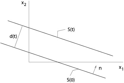
here we assume that $0$ is in he range of $f:\ \mathbb{R}^1\mapsto\mathbb{R}^1$. Thus, $\mathcal{S}(t)$ is defined by $n\cdot x-Vt=c$, where $c$ is a fixed constant. It follows that the planes $\mathcal{S}(t)$ with normal $n$ move with speed $V$ in direction of $n$, see Figure 3.3.1.1.

Figure 3.3.1.1: $d'(t)$ is the speed of plane waves

$V$ is called speed of the plane wave $\mathcal{S}(t)$.

Remark. According to the previous discussions, singularities of a solution of Maxwell equations are located at most on characteristic surfaces.

A special case of Maxwell equations are the telegraph equations, which follow from Maxwell equations if $\text{\div}\ E=0$ and $\text{div}\ H=0$$ i. e., $E$ and $H$ are fields free of sources. In fact, it is sufficient to assume that this assumption is satisfied at a fixed time $t_0$ only, see an exercise.

Since

$$
\text{rot}_x\ \text{rot}_x\ A=\mbox{grad}_x\ \text{div}_x\ A-\triangle_xA
\]

for each $C^2$-vector field $A$, it follows from Maxwell equations the uncoupled system

$$\begin{eqnarray*} \triangle_xE&=&\frac{\epsilon\mu}{c^2}E_{tt}+\frac{\lambda\mu}{c^2}E_t\\ \triangle_xH&=&\frac{\epsilon\mu}{c^2}H_{tt}+\frac{\lambda\mu}{c^2}H_t. \end{eqnarray*}$$

Example 3.3.1.3: Equations of Gas Dynamics

Consider the following quasilinear equations of first order.

$$
v_t+(v\cdot\nabla_x)\ v+\frac{1}{\rho} \nabla_x p =f\ \ \ \mbox{(Euler equations)}.
\]

Here is

• $v=(v_1,v_2,v_3)$ the vector of speed, $v_i=v_i(x,t)$, $x=(x_1,x_2,x_3)$,
• $p$ pressure, $p=(x,t)$,
• $\rho$ density, $\rho=\rho(x,t)$,
• $f=(f_1,f_2,f_3)$ density of the external force, $f_i=f_i(x,t)$,

$(v\cdot\nabla_x)v\equiv (v\cdot\nabla_x v_1,v\cdot\nabla_x v_2,v\cdot\nabla_x v_3))^T$.

The second equation is

$$
\rho_t+v\cdot\nabla_x\rho+\rho\ \text{div}_x\ v=0\ \ \ \mbox{(conservation of mass)}.
\]

Assume the gas is compressible and that there is a function (state equation)

$$
p=p(\rho),
\]

where $p'(\rho)>0$ if $\rho>0$. Then the above system of four equations is

$$\begin{eqnarray} \label{euler}\tag{3.3.1.5} v_t+(v\cdot\nabla)v+\frac{1}{\rho}p'(\rho)\nabla\rho&=&f\\ \label{cont}\tag{3.3.1.6} \rho_t+ \rho\ \text{div}\ v+v\cdot\nabla\rho&=&0, \end{eqnarray}$$

where $\nabla\equiv\nabla_x$ and $\text{div}\equiv\text{div}_x$, i. e., these operators apply on the spatial variables only.

The characteristic differential equation is here
$$
\left| $$\begin{array}{cccc} \frac{d\chi}{dt}&0&0&\frac{1}{\rho}p'\chi_{x_1}\\ 0&\frac{d\chi}{dt}&0&\frac{1}{\rho}p'\chi_{x_2}\\ 0&0&\frac{d\chi}{dt}&\frac{1}{\rho}p'\chi_{x_3}\\ \rho\chi_{x_1}& \rho\chi_{x_2}&\rho\chi_{x_3}&\frac{d\chi}{dt} \end{array}$$ \right|=0,
\]

where

$$\dfrac{d\chi}{dt}:=\chi_t+(\nabla_x\chi)\cdot v. \]

Evaluating the determinant, we get the characteristic differential equation

$$\begin{equation} \label{chargas}\tag{3.3.1.7} \left(\frac{d\chi}{dt}\right)^2\left(\left(\frac{d\chi}{dt}\right)^2-p'(\rho)|\nabla_x\chi|^2\right)=0. \end{equation}$$

This equation implies consequences for the speed of the characteristic surfaces as the following consideration shows.

Consider a family $\mathcal{S}(t)$ of surfaces in $\mathbb{R}^3$ defined by $\chi(x,t)=c$, where
$x\in\mathbb{R}^3$ and $c$ is a fixed constant. As usually, we assume that $\nabla_x\chi\not=0$.
One of the two normals on $\mathcal{S}(t)$ at a point of the surface $\mathcal{S}(t)$ is given by, see an exercise,
$$\begin{equation} \label{surfnormal}\tag{3.3.1.8} {\bf n}=\frac{\nabla_x\chi}{|\nabla_x\chi|}. \end{equation}$$
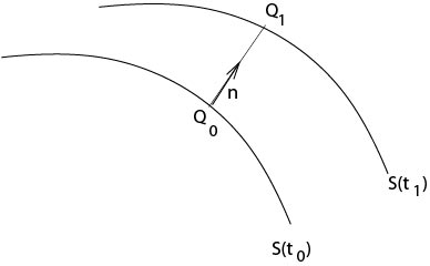
Let $Q_0\in\mathcal{S}(t_0)$ and let $Q_1\in\mathcal{S}(t_1)$ be a point on the line defined by $Q_0+s{\bf n}$, where ${\bf n}$ is the normal ($\ref{surfnormal}$) on $\mathcal{S}(t_0)$ at $Q_0$ and $t_0<t_1$, $t_1-t_0$ small, see Figure 3.3.1.2.

3.3.1.2: Definition of the speed of a surface

Definition. The limit
$$P=\lim_{t_1\to t_0}\frac{|Q_1-Q_0|}{t_1-t_0}$$
is called speed of the surface $\mathcal{S}(t)$.

Proposition 3.2. The speed of the surface $\mathcal{S}(t)$ is
$$\begin{equation} \label{speedsurf} P=-\frac{\chi_t}{|\nabla_x\chi|}. \end{equation}$$

Proof. The proof follows from $\chi(Q_0,t_0)=0$ and $\chi(Q_0+d{\bf n},t_0+\triangle t)=0$, where $d=|Q_1-Q_0|$ and $\triangle t=t_1-t_0$.

$\Box$

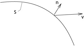
Set $v_n:=v\cdot{\bf n}$ which is the component of the velocity vector in direction ${\bf n}$.
From ({$\ref{surfnormal}$) we get
$$
v_n=\frac{1}{|\nabla_x\chi|}v\cdot \nabla_x\chi.
\]

Definition. $V:=P-v_n$, the difference of the speed of the surface and the speed of liquid particles, is called relative speed.

Figure 3.3.1.3: Definition of relative speed

Using the above formulas for $P$ and $v_n$ it follows
$$V=P-v_n=-\frac{\chi_t}{|\nabla_x\chi|}-\frac{v\cdot\nabla_x\chi}{|\nabla_x\chi|}=-\frac{1}{|\nabla_x\chi|}\frac{d\chi}{dt}.$$
Then, we obtain from the characteristic equation ($\ref{chargas}$) that
$$V^2|\nabla_x\chi|^2\left(V^2|\nabla_x\chi|^2-p'(\rho)|\nabla_x\chi|^2\right)=0.$$
An interesting conclusion is that there are two relative speeds: $V=0$ or $V^2=p'(\rho)$.

Definition. $\sqrt{p'(\rho)}$ is called speed of sound.

Contributors and Attributions

• Prof. Dr. Erich Miersemann (Universität Leipzig)

• Integrated by Justin Marshall.