
4.2: Analytic Geometry Proof
- Page ID
- 104978

We have been doing what is known as "synthetic" proof, proving theorems directly from the axioms entirely in the abstract (in spite of the somewhat unorthodox approach of acknowledging that we never formally state these axioms instead of the usual, lying about it). The pictures we draw are helpful but meaningless unless we accept the idealized plane of a blackboard or sheet of paper (and associated points, lines, and the like) as a model for the abstract geometry that is intended to be strictly conceptual. Another model that we have been trained to believe is exactly the same thing is the Cartesian plane. In fact, this is an entirely separate model that has nothing in common with our usual plane except for our conviction that they are one and the same. In fact, they are very different. In another sense, however, they are the same; that is the nature of the axioms for Euclidean geometry being "categorical" introduced in the Introduction. The idea is that a proof in one model of Euclidean geometry can be identified completely (what are points, lines, etc.) in any other model or in the abstract "model-free" situation and the proof will be equally valid. That is, a Cartesian plane proof really is a valid proof. Although some of the full geometry (especially in n-dimensional Euclidean space) are better handled with vector notation (angle congruence for example), we are trying to present the situation at the lowest level possible for the most basic understanding.
Recall that when introducing the Poincaré disk model for hyperbolic geometry, we started off with the model being a triple, \(\mathcal{L}=(\theta, L, C)\), for the set of points of the geometry, the subsets to be called lines, and the subsets to be called circles. We were "fudging" a little in that the concept for segment length (distance between 2 points needed to prove the Ruler Postulate) meant that "circles" already had a definition as the set of all points equidistant from some point called its center. The problem was that we had not developed much feeling for Poincaré distance (still have not, truth be told!). In this "new" situation, Euclidean distance is not a problem, the traditional distance formula, so \(l=(0, L)\) where:
\(p=\left\{(\mathrm{x}, \mathrm{y}) \mid \mathrm{x}, \mathrm{y}\right.\) the set of all ordered pairs, \(\left.\mathbf{R} \times \mathbf{R}=\mathbf{R}^{2}\right\}\)
\(\mathcal{L}=\left\{\ell \mid l=\{(x, y) \mid a x+b y=c\}\right.\) for some \(\left.a, b, c \in \mathbf{R}, a^{2}+b^{2}>0\right\}\) (i.e., not both \(a=0\) and \(\left.b=0\right)\).
That is, a line is just the set of all solutions to any "linear equation" (even the words we use are tilting the pinball table!). In this Cartesian product setting, we are so used to identifying each ordered pair as a unique point in the coordinate plane that we have to force ourselves to think that its being nothing more than a left parenthesis "(" followed by two real numbers separated by a comma and a right parenthesis. Even Euclidean 3-space makes the identification obvious albeit harder to sketch. To get a better idea, think of a point in \(\mathbf{R}^{\mathrm{n}}\) for \(\mathrm{n} \geq 4\) and see if the identification remains as clear. To confirm that it is a model for Euclidean plane geometry when \(n=2\), we would have to prove all of the axioms as theorems but, in fact, some of them we’ve been doing ever since Algebra 1! For example, proof of Axiom 1 is nothing more than finding the (being more careful, "an") equation that is satisfied by two given pairs of ordered pairs and confirming that any linear equation that is satisfied by these two pairs has exactly the same set of solutions (same solution set). That is just a standard Algebra I problem if done in terms of general coefficients \(\mathrm{P}_{1}\left(\mathrm{x}_{1}, \mathrm{y}_{1}\right) \neq \mathrm{P}_{2}\left(\mathrm{x}_{2}, \mathrm{y}_{2}\right)\) taking into account the special cases of \(\mathrm{x}_{1}=\mathrm{x}_{2}\) exclusive or \(\mathrm{y}_{1}=\mathrm{y}_{2}\). However, considering this model for Euclidean geometry in such a formal way would defeat the purpose. The whole idea is to use our close identification of the Cartesian plane (coordinate axes on the conventional plane) to give an alternate, sometimes simpler, proof.
The distance between two points is just the Pythagorean theorem-based distance formula. Angles are a little trickier but usually don’t show up in the kinds of proofs that are easily constructed "analytically". For lines that are neither parallel to the \(\mathrm{x}\)-axis or to the \(\mathrm{y}\)-axis, it is easy to prove that distinct lines are parallel (no points in common) if and only if they have the same slope as long as we extend parallel to include the equivalence property "reflexivity" idea that a line be defined to be parallel to itself. Similarly, it is easy to prove that lines are perpendicular if and only if their slopes are negative reciprocals of each other (product is -1) along with the special case of parallels to the coordinate axes. Note: This is not a definition perpendicular already has defined meaning - this is a theorem. The measure of angles is most easily done with vector notation. We won’t need it but for completeness sake:
The measure of the angle between two vectors \(u\) and \(v\) at the origin is \(\alpha=\cos ^{-1}(u \cdot v /\|u\|\|V\|)\), the size of an angle with cosine being the dot product of the vectors divided by the product of their lengths so for general \(\angle \mathrm{BAC}\) with \(\mathrm{B}\left(\mathrm{x}_{\mathrm{B}}, \mathrm{y}_{\mathrm{B}}\right), \mathrm{A}\left(\mathrm{x}_{\mathrm{A}}, \mathrm{y}_{\mathrm{A}}\right)\), and \(C\left(\mathrm{x}_{\mathrm{C}}, \mathrm{y}_{\mathrm{C}}\right)\):
\[m(\angle B A C)=\cos ^{-1}\left(\frac{\left(x_{B}-x_{A}\right)\left(x_{C}-x_{A}\right)+\left(y_{B}-x_{A}\right)\left(y_{C}-x_{A}\right)}{\left(\sqrt{\left(x_{B}-x_{A}\right)^{2}+\left(y_{B}-x_{A}\right)^{2}}\right)\left(\sqrt{\left(x_{C}-x_{A}\right)^{2}+\left(y_{C}-x_{A}\right)^{2}}\right)}\right) \nonumber \]
This was expressed in terms of the plane \(\left(\mathbf{R}^{n}\right.\) where \(\left.n=2\right)\) but the same vector approach is valid for any \(n\). That is, the same vector formula for the measure of an angle for \(\mathbf{R}^{\mathrm{n}}\) for any \(\mathrm{n}\).
Instead of more of the details, here is an example of a theorem proved synthetically now using an analytic proof. Examples of other theorems are given in PS 4, #27 and #28.
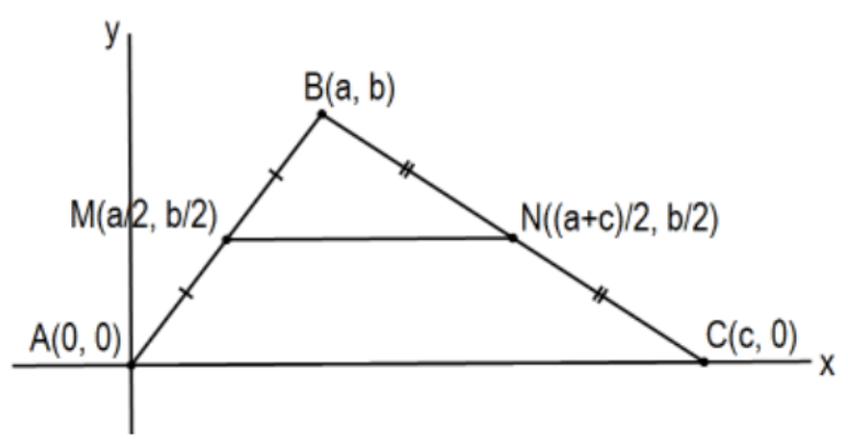
The line determined by the midpoints of two sides of a triangle is parallel to the third side and the length of its segment is half of that third side.
Proof: In order to minimize algebraic complexity, it is very helpful to coordinate the plane in such a way as to make the algebraic arithmetic as easy as possible being careful, of course, to be completely general in the assignment. A common simplification is with one side of a figure being studied along the \(x\)-axis and an important point \((0,0)\). In this case, a reasonable place to start would be for our general triangle to be \(\triangle \mathrm{ABC}\) with ordered pair vertices \(\mathrm{A}(0,0), \mathrm{B}(\mathrm{a}, \mathrm{b})\), and \(\mathrm{C}(\mathrm{c}, 0)\) with \(\mathrm{b} \neq 0\) and \(\mathrm{c} \neq 0\) as pictured. [Even easier would have been \(\mathrm{A}(\mathrm{a}, 0), \mathrm{B}(0, \mathrm{~b})\), and \(\mathrm{C}(\mathrm{c}, 0)\) with \(\mathrm{b} \neq 0\) and \(\mathrm{a} \neq \mathrm{c}\).] Of course, this assumes that calculation of a segment’s midpoint is known but writing an equation for line MN \((\mathrm{y}=\mathrm{b} / 2)\) to confirm that it is parallel to the \(\mathrm{x}\)-axis \((\mathrm{y}=0)\) is a triviality as is calculating the length of segment \(M N\) and confirming that it is half the length of segment AC. QED.
Note: This is so simple that it almost feels like we are cheating but it is a perfectly valid proof assuming the fact that the axioms for Euclidean geometry are categorical and that this is a model for Euclidean geometry.