
8.1: Polar Coordinates and Polar Graphs
- Page ID
- 14545

\( \newcommand{\vecs}[1]{\overset { \scriptstyle \rightharpoonup} {\mathbf{#1}} } \)
\( \newcommand{\vecd}[1]{\overset{-\!-\!\rightharpoonup}{\vphantom{a}\smash {#1}}} \)
\( \newcommand{\id}{\mathrm{id}}\) \( \newcommand{\Span}{\mathrm{span}}\)
( \newcommand{\kernel}{\mathrm{null}\,}\) \( \newcommand{\range}{\mathrm{range}\,}\)
\( \newcommand{\RealPart}{\mathrm{Re}}\) \( \newcommand{\ImaginaryPart}{\mathrm{Im}}\)
\( \newcommand{\Argument}{\mathrm{Arg}}\) \( \newcommand{\norm}[1]{\| #1 \|}\)
\( \newcommand{\inner}[2]{\langle #1, #2 \rangle}\)
\( \newcommand{\Span}{\mathrm{span}}\)
\( \newcommand{\id}{\mathrm{id}}\)
\( \newcommand{\Span}{\mathrm{span}}\)
\( \newcommand{\kernel}{\mathrm{null}\,}\)
\( \newcommand{\range}{\mathrm{range}\,}\)
\( \newcommand{\RealPart}{\mathrm{Re}}\)
\( \newcommand{\ImaginaryPart}{\mathrm{Im}}\)
\( \newcommand{\Argument}{\mathrm{Arg}}\)
\( \newcommand{\norm}[1]{\| #1 \|}\)
\( \newcommand{\inner}[2]{\langle #1, #2 \rangle}\)
\( \newcommand{\Span}{\mathrm{span}}\) \( \newcommand{\AA}{\unicode[.8,0]{x212B}}\)
\( \newcommand{\vectorA}[1]{\vec{#1}} % arrow\)
\( \newcommand{\vectorAt}[1]{\vec{\text{#1}}} % arrow\)
\( \newcommand{\vectorB}[1]{\overset { \scriptstyle \rightharpoonup} {\mathbf{#1}} } \)
\( \newcommand{\vectorC}[1]{\textbf{#1}} \)
\( \newcommand{\vectorD}[1]{\overrightarrow{#1}} \)
\( \newcommand{\vectorDt}[1]{\overrightarrow{\text{#1}}} \)
\( \newcommand{\vectE}[1]{\overset{-\!-\!\rightharpoonup}{\vphantom{a}\smash{\mathbf {#1}}}} \)
\( \newcommand{\vecs}[1]{\overset { \scriptstyle \rightharpoonup} {\mathbf{#1}} } \)
\( \newcommand{\vecd}[1]{\overset{-\!-\!\rightharpoonup}{\vphantom{a}\smash {#1}}} \)
\(\newcommand{\avec}{\mathbf a}\) \(\newcommand{\bvec}{\mathbf b}\) \(\newcommand{\cvec}{\mathbf c}\) \(\newcommand{\dvec}{\mathbf d}\) \(\newcommand{\dtil}{\widetilde{\mathbf d}}\) \(\newcommand{\evec}{\mathbf e}\) \(\newcommand{\fvec}{\mathbf f}\) \(\newcommand{\nvec}{\mathbf n}\) \(\newcommand{\pvec}{\mathbf p}\) \(\newcommand{\qvec}{\mathbf q}\) \(\newcommand{\svec}{\mathbf s}\) \(\newcommand{\tvec}{\mathbf t}\) \(\newcommand{\uvec}{\mathbf u}\) \(\newcommand{\vvec}{\mathbf v}\) \(\newcommand{\wvec}{\mathbf w}\) \(\newcommand{\xvec}{\mathbf x}\) \(\newcommand{\yvec}{\mathbf y}\) \(\newcommand{\zvec}{\mathbf z}\) \(\newcommand{\rvec}{\mathbf r}\) \(\newcommand{\mvec}{\mathbf m}\) \(\newcommand{\zerovec}{\mathbf 0}\) \(\newcommand{\onevec}{\mathbf 1}\) \(\newcommand{\real}{\mathbb R}\) \(\newcommand{\twovec}[2]{\left[\begin{array}{r}#1 \\ #2 \end{array}\right]}\) \(\newcommand{\ctwovec}[2]{\left[\begin{array}{c}#1 \\ #2 \end{array}\right]}\) \(\newcommand{\threevec}[3]{\left[\begin{array}{r}#1 \\ #2 \\ #3 \end{array}\right]}\) \(\newcommand{\cthreevec}[3]{\left[\begin{array}{c}#1 \\ #2 \\ #3 \end{array}\right]}\) \(\newcommand{\fourvec}[4]{\left[\begin{array}{r}#1 \\ #2 \\ #3 \\ #4 \end{array}\right]}\) \(\newcommand{\cfourvec}[4]{\left[\begin{array}{c}#1 \\ #2 \\ #3 \\ #4 \end{array}\right]}\) \(\newcommand{\fivevec}[5]{\left[\begin{array}{r}#1 \\ #2 \\ #3 \\ #4 \\ #5 \\ \end{array}\right]}\) \(\newcommand{\cfivevec}[5]{\left[\begin{array}{c}#1 \\ #2 \\ #3 \\ #4 \\ #5 \\ \end{array}\right]}\) \(\newcommand{\mattwo}[4]{\left[\begin{array}{rr}#1 \amp #2 \\ #3 \amp #4 \\ \end{array}\right]}\) \(\newcommand{\laspan}[1]{\text{Span}\{#1\}}\) \(\newcommand{\bcal}{\cal B}\) \(\newcommand{\ccal}{\cal C}\) \(\newcommand{\scal}{\cal S}\) \(\newcommand{\wcal}{\cal W}\) \(\newcommand{\ecal}{\cal E}\) \(\newcommand{\coords}[2]{\left\{#1\right\}_{#2}}\) \(\newcommand{\gray}[1]{\color{gray}{#1}}\) \(\newcommand{\lgray}[1]{\color{lightgray}{#1}}\) \(\newcommand{\rank}{\operatorname{rank}}\) \(\newcommand{\row}{\text{Row}}\) \(\newcommand{\col}{\text{Col}}\) \(\renewcommand{\row}{\text{Row}}\) \(\newcommand{\nul}{\text{Nul}}\) \(\newcommand{\var}{\text{Var}}\) \(\newcommand{\corr}{\text{corr}}\) \(\newcommand{\len}[1]{\left|#1\right|}\) \(\newcommand{\bbar}{\overline{\bvec}}\) \(\newcommand{\bhat}{\widehat{\bvec}}\) \(\newcommand{\bperp}{\bvec^\perp}\) \(\newcommand{\xhat}{\widehat{\xvec}}\) \(\newcommand{\vhat}{\widehat{\vvec}}\) \(\newcommand{\uhat}{\widehat{\uvec}}\) \(\newcommand{\what}{\widehat{\wvec}}\) \(\newcommand{\Sighat}{\widehat{\Sigma}}\) \(\newcommand{\lt}{<}\) \(\newcommand{\gt}{>}\) \(\newcommand{\amp}{&}\) \(\definecolor{fillinmathshade}{gray}{0.9}\)- Understand polar coordinates.
- Convert points between Cartesian and polar coordinates.
You have likely encountered the Cartesian coordinate system in many aspects of mathematics. There is an alternative way to represent points in space, called polar coordinates. The idea is suggested in the following picture.
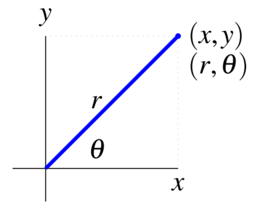
Consider the point above, which would be specified as \((x,y)\) in Cartesian coordinates. We can also specify this point using polar coordinates, which we write as \(\left( r, \theta \right)\). The number \(r\) is the distance from the origin\(\left( 0,0\right)\) to the point, while \(\theta\) is the angle shown between the positive \(x\) axis and the line from the origin to the point. In this way, the point can be specified in polar coordinates as \(\left(r, \theta \right)\).
Now suppose we are given an ordered pair \(\left( r,\theta \right)\) where \(r\) and \(\theta\) are real numbers. We want to determine the point specified by this ordered pair. We can use \(\theta\) to identify a ray from the origin as follows. Let the ray pass from \(\left( 0,0\right)\) through the point \(\left( \cos \theta ,\sin \theta \right)\) as shown.
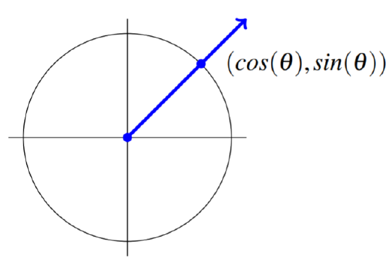
The ray is identified on the graph as the line from the origin, through the point \((\mbox{cos}(\theta),\mbox{sin}(\theta))\). Now if \(r>0,\) go a distance equal to \(r\) in the direction of the displayed arrow starting at \((0,0)\). If \(r<0,\) move in the opposite direction a distance of \(\left\vert r\right\vert\). This is the point determined by \(\left( r,\theta \right)\).
It is common to assume that \(\theta\) is in the interval \([0,2\pi )\) and \(r>0.\) In this case, there is a very simple relationship between the Cartesian and polar coordinates, given by \[x=r\cos \left( \theta \right) ,\ \ y=r\sin \left( \theta \right) \label{cartpolcoord}\]
These equations demonstrate how to find the Cartesian coordinates when we are given the polar coordinates of a point. They can also be used to find the polar coordinates when we know \(\left( x, y \right)\). A simpler way to do this is the following equations: \[\begin{array}{l} r = \sqrt{x^2 + y^2} \\ \\ \mbox{tan} \left(\theta\right) = \frac{y}{x} \end{array} \label{polcartcoord}\]
In the next example, we look at how to find the Cartesian coordinates of a point specified by polar coordinates.
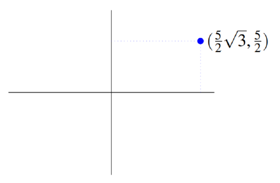
The polar coordinates of a point in the plane are \(\left( 5,\pi /6\right)\). Find the Cartesian coordinates of this point.
Solution
The point is specified by the polar coordinates \(\left( 5,\pi /6\right)\). Therefore \(r=5\) and \(\theta = \pi /6\). From \(\eqref{cartpolcoord}\) \[x= r \cos \left( \theta \right)= 5\cos \left( \frac{\pi }{6}\right) = \frac{5}{2}\sqrt{3}\nonumber \] \[y= r \sin \left( \theta \right) = 5\sin \left( \frac{\pi }{6}\right) = \frac{5}{2}\nonumber \] Thus the Cartesian coordinates are \(\left( \frac{5}{2}\sqrt{3}, \frac{5}{2}\right)\). The point is shown in the below graph.
Consider the following example of the case where \(r < 0\).
The polar coordinates of a point in the plane are \(\left( -5,\pi /6\right) .\) Find the Cartesian coordinates.
Solution
For the point specified by the polar coordinates \(\left( -5, \pi /6 \right)\), \(r=-5\), and \(x\theta = \pi /6\). From \(\eqref{cartpolcoord}\) \[x= r \cos \left( \theta \right)= -5\cos \left( \frac{\pi }{6}\right) = -\frac{5}{2}\sqrt{3}\nonumber \] \[y= r \sin \left( \theta \right) = -5\sin \left( \frac{\pi }{6}\right) = -\frac{5}{2}\nonumber \] Thus the Cartesian coordinates are \(\left( -\frac{5}{2}\sqrt{3}, -\frac{5}{2}\right)\). The point is shown in the following graph.
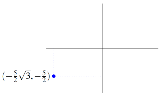
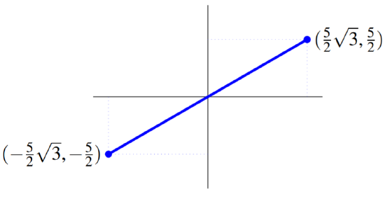
Recall from the previous example that for the point specified by \(\left( 5, \pi /6 \right)\), the Cartesian coordinates are \(\left( \frac{5}{2}\sqrt{3}, \frac{5}{2}\right)\). Notice that in this example, by multiplying \(r\) by \(-1\), the resulting Cartesian coordinates are also multiplied by \(-1\).
The following picture exhibits both points in the above two examples to emphasize how they are just on opposite sides of \(\left( 0,0\right)\) but at the same distance from \(\left( 0,0\right)\).
In the next two examples, we look at how to convert Cartesian coordinates to polar coordinates.
Suppose the Cartesian coordinates of a point are \(\left( 3,4\right)\). Find a pair of polar coordinates which correspond to this point.
Solution
Using equation \(\eqref{polcartcoord}\), we can find \(r\) and \(\theta\). Hence \(r=\sqrt{3^{2}+4^{2}}=5\). It remains to identify the angle \(\theta\) between the positive \(x\) axis and the line from the origin to the point. Since both the \(x\) and \(y\) values are positive, the point is in the first quadrant. Therefore, \(\theta\) is between \(0\) and \(\pi /2\ \). Using this and \(\eqref{polcartcoord}\), we have to solve: \[\mbox{tan}\left(\theta \right)=\frac{4}{3}\nonumber \] Conversely, we can use equation \(\eqref{cartpolcoord}\) as follows: \[3=5\cos \left( \theta \right)\nonumber \] \[4 = 5\sin \left( \theta \right)\nonumber \] Solving these equations, we find that, approximately, \(\theta =0.\, 927\,295\) radians.
Consider the following example.
Suppose the Cartesian coordinates of a point are \(\left( -\sqrt{3},1\right)\). Find the polar coordinates which correspond to this point.
Solution
Given the point \(\left( -\sqrt{3}, 1\right)\), \[\begin{aligned} r &= \sqrt{ 1^2 + (-\sqrt{3})^2}\\ &= \sqrt{1 + 3}\\ &=2\end{aligned}\] In this case, the point is in the second quadrant since the \(x\) value is negative and the \(y\) value is positive. Therefore, \(\theta\) will be between \(\pi/2\) and \(\pi\). Solving the equations \[-\sqrt{3}= 2 \cos \left(\theta\right)\nonumber \] \[1 = 2 \sin \left( \theta\right)\nonumber \] we find that \(\theta = 5\pi /6.\) Hence the polar coordinates for this point are \(\left(2, 5\pi /6 \right)\).
Consider this example. Suppose we used \(r=-2\) and \(\theta =2\pi -\left( \pi /6\right) = 11\pi /6\). These coordinates specify the same point as above. Observe that there are infinitely many ways to identify this particular point with polar coordinates. In fact, every point can be represented with polar coordinates in infinitely many ways. Because of this, it will usually be the case that \(\theta\) is confined to lie in some interval of length \(2\pi\) and \(r>0\), for real numbers \(r\) and \(\theta\).
Just as with Cartesian coordinates, it is possible to use relations between the polar coordinates to specify points in the plane. The process of sketching the graphs of these relations is very similar to that used to sketch graphs of functions in Cartesian coordinates. Consider a relation between polar coordinates of the form, \(r=f\left( \theta \right)\). To graph such a relation, first make a table of the form
| \(\theta\) | \(r\) |
|---|---|
| \(\theta_1\) | \(f(\theta_1)\) |
| \(\theta_2\) | \(f(\theta_2)\) |
| \(\vdots\) | \(\vdots\) |
Graph the resulting points and connect them with a curve. The following picture illustrates how to begin this process.
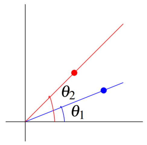
To find the point in the plane corresponding to the ordered pair \(\left( f\left( \theta \right) ,\theta \right)\), we follow the same process as when finding the point corresponding to \(\left( r, \theta \right)\).
Consider the following example of this procedure, incorporating computer software.
Graphing a Polar Equation Graph the polar equation \(r=1+\cos \theta\).
Solution
We will use the computer software Maple to complete this example. The command which produces the polar graph of the above equation is: \(>\) plot(1+cos(t),t= 0..2*Pi,coords=polar). Here we use \(t\) to represent the variable \(\theta\) for convenience. The command tells Maple that \(r\) is given by \(1+\cos \left( t\right)\) and that \(t\in \left[ 0,2\pi \right]\).
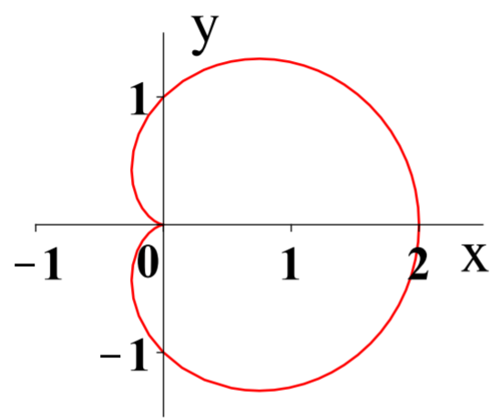
The above graph makes sense when considered in terms of trigonometric functions. Suppose \(\theta =0,r=2\) and let \(\theta\) increase to \(\pi /2\). As \(\theta\) increases, \(\cos \theta\) decreases to 0. Thus the line from the origin to the point on the curve should get shorter as \(\theta\) goes from \(0\) to \(\pi /2\). As \(\theta\) goes from \(\pi /2\) to \(\pi\), \(\cos \theta\) decreases, eventually equaling \(-1\) at \(\theta =\pi\). Thus \(r=0\) at this point. This scenario is depicted in the above graph, which shows a function called a cardioid.
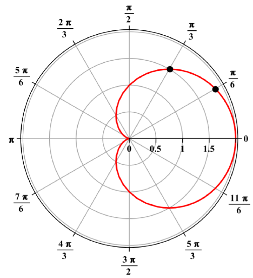
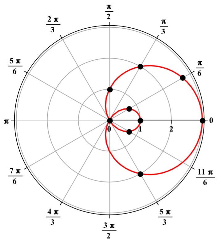
The following picture illustrates the above procedure for obtaining the polar graph of \(r=1+cos(\theta)\). In this picture, the concentric circles correspond to values of \(r\) while the rays from the origin correspond to the angles which are shown on the picture. The dot on the ray corresponding to the angle \(\pi/6\) is located at a distance of \(r = 1+cos(\pi/6)\) from the origin. The dot on the ray corresponding to the angle \(\pi/3\) is located at a distance of \(r = 1+cos(\pi/3)\) from the origin and so forth. The polar graph is obtained by connecting such points with a smooth curve, with the result being the figure shown above.
Consider another example of constructing a polar graph.
Graph \(r=1+2\cos \theta\) for \(\theta \in \left[ 0,2\pi \right]\).
Solution
The graph of the polar equation \(r=1+2\cos \theta\) for \(\theta \in \left[ 0,2\pi \right]\) is given as follows.
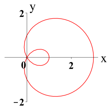
To see the way this is graphed, consider the following picture. First the indicated points were graphed and then the curve was drawn to connect the points. When done by a computer, many more points are used to create a more accurate picture.
Consider first the following table of points.
| \(\theta\) | \(\pi /6\) | \(\pi /3\) | \(\pi /2\) | \(5\pi /6\) | \(\pi\) | \(4\pi /3\) | \(7\pi /6\) | \(5\pi /3\) |
|---|---|---|---|---|---|---|---|---|
| \(r\) | \(\sqrt{3}+1\) | \(2\) | \(1\) | \(1-\sqrt{3}\) | \(-1\) | \(0\) | \(1-\sqrt{3}\) | \(2\) |
Note how some entries in the table have \(r<0.\) To graph these points, simply move in the opposite direction. These types of points are responsible for the small loop on the inside of the larger loop in the graph.
The process of constructing these graphs can be greatly facilitated by computer software. However, the use of such software should not replace understanding the steps involved.
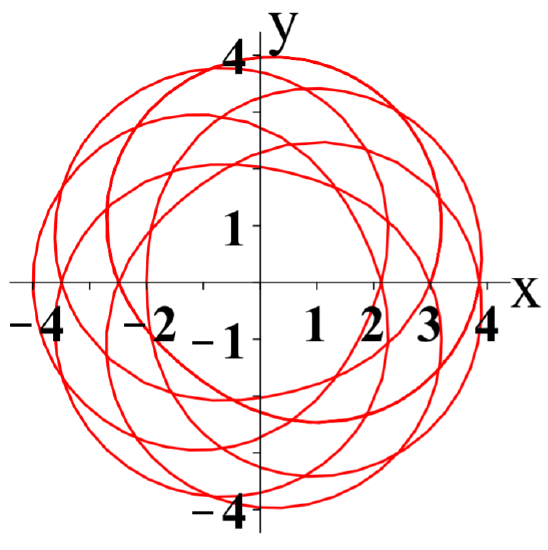
The next example shows the graph for the equation \(r=3+\sin \left( \displaystyle \frac{7\theta }{6}\right)\). For complicated polar graphs, computer software is used to facilitate the process.
Graph \(r=3+\sin \left( \displaystyle \frac{7\theta }{6} \right)\) for \(\theta \in \left[ 0,14\pi \right]\).
Solution
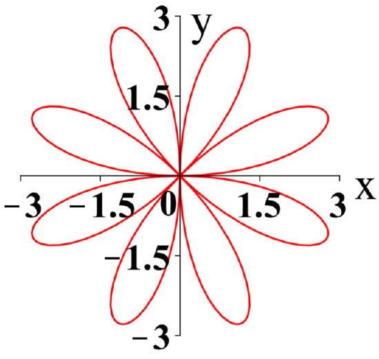
The next example shows another situation in which \(r\) can be negative.
Graph \(r=3sin(4\theta)\) for \(\theta \in \left[ 0,2\pi \right]\).
Solution
We conclude this section with an interesting graph of a simple polar equation.
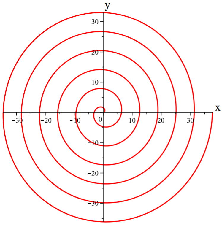
Graph \(r=\theta\) for \(\theta \in [0,2\pi]\).
Solution
The graph of this polar equation is a spiral. This is the case because as \(\theta\) increases, so does \(r\).
In the next section, we will look at two ways of generalizing polar coordinates to three dimensions.