1: What is linear algebra
- Page ID
- 319
\( \newcommand{\vecs}[1]{\overset { \scriptstyle \rightharpoonup} {\mathbf{#1}} } \)
\( \newcommand{\vecd}[1]{\overset{-\!-\!\rightharpoonup}{\vphantom{a}\smash {#1}}} \)
\( \newcommand{\dsum}{\displaystyle\sum\limits} \)
\( \newcommand{\dint}{\displaystyle\int\limits} \)
\( \newcommand{\dlim}{\displaystyle\lim\limits} \)
\( \newcommand{\id}{\mathrm{id}}\) \( \newcommand{\Span}{\mathrm{span}}\)
( \newcommand{\kernel}{\mathrm{null}\,}\) \( \newcommand{\range}{\mathrm{range}\,}\)
\( \newcommand{\RealPart}{\mathrm{Re}}\) \( \newcommand{\ImaginaryPart}{\mathrm{Im}}\)
\( \newcommand{\Argument}{\mathrm{Arg}}\) \( \newcommand{\norm}[1]{\| #1 \|}\)
\( \newcommand{\inner}[2]{\langle #1, #2 \rangle}\)
\( \newcommand{\Span}{\mathrm{span}}\)
\( \newcommand{\id}{\mathrm{id}}\)
\( \newcommand{\Span}{\mathrm{span}}\)
\( \newcommand{\kernel}{\mathrm{null}\,}\)
\( \newcommand{\range}{\mathrm{range}\,}\)
\( \newcommand{\RealPart}{\mathrm{Re}}\)
\( \newcommand{\ImaginaryPart}{\mathrm{Im}}\)
\( \newcommand{\Argument}{\mathrm{Arg}}\)
\( \newcommand{\norm}[1]{\| #1 \|}\)
\( \newcommand{\inner}[2]{\langle #1, #2 \rangle}\)
\( \newcommand{\Span}{\mathrm{span}}\) \( \newcommand{\AA}{\unicode[.8,0]{x212B}}\)
\( \newcommand{\vectorA}[1]{\vec{#1}} % arrow\)
\( \newcommand{\vectorAt}[1]{\vec{\text{#1}}} % arrow\)
\( \newcommand{\vectorB}[1]{\overset { \scriptstyle \rightharpoonup} {\mathbf{#1}} } \)
\( \newcommand{\vectorC}[1]{\textbf{#1}} \)
\( \newcommand{\vectorD}[1]{\overrightarrow{#1}} \)
\( \newcommand{\vectorDt}[1]{\overrightarrow{\text{#1}}} \)
\( \newcommand{\vectE}[1]{\overset{-\!-\!\rightharpoonup}{\vphantom{a}\smash{\mathbf {#1}}}} \)
\( \newcommand{\vecs}[1]{\overset { \scriptstyle \rightharpoonup} {\mathbf{#1}} } \)
\(\newcommand{\longvect}{\overrightarrow}\)
\( \newcommand{\vecd}[1]{\overset{-\!-\!\rightharpoonup}{\vphantom{a}\smash {#1}}} \)
\(\newcommand{\avec}{\mathbf a}\) \(\newcommand{\bvec}{\mathbf b}\) \(\newcommand{\cvec}{\mathbf c}\) \(\newcommand{\dvec}{\mathbf d}\) \(\newcommand{\dtil}{\widetilde{\mathbf d}}\) \(\newcommand{\evec}{\mathbf e}\) \(\newcommand{\fvec}{\mathbf f}\) \(\newcommand{\nvec}{\mathbf n}\) \(\newcommand{\pvec}{\mathbf p}\) \(\newcommand{\qvec}{\mathbf q}\) \(\newcommand{\svec}{\mathbf s}\) \(\newcommand{\tvec}{\mathbf t}\) \(\newcommand{\uvec}{\mathbf u}\) \(\newcommand{\vvec}{\mathbf v}\) \(\newcommand{\wvec}{\mathbf w}\) \(\newcommand{\xvec}{\mathbf x}\) \(\newcommand{\yvec}{\mathbf y}\) \(\newcommand{\zvec}{\mathbf z}\) \(\newcommand{\rvec}{\mathbf r}\) \(\newcommand{\mvec}{\mathbf m}\) \(\newcommand{\zerovec}{\mathbf 0}\) \(\newcommand{\onevec}{\mathbf 1}\) \(\newcommand{\real}{\mathbb R}\) \(\newcommand{\twovec}[2]{\left[\begin{array}{r}#1 \\ #2 \end{array}\right]}\) \(\newcommand{\ctwovec}[2]{\left[\begin{array}{c}#1 \\ #2 \end{array}\right]}\) \(\newcommand{\threevec}[3]{\left[\begin{array}{r}#1 \\ #2 \\ #3 \end{array}\right]}\) \(\newcommand{\cthreevec}[3]{\left[\begin{array}{c}#1 \\ #2 \\ #3 \end{array}\right]}\) \(\newcommand{\fourvec}[4]{\left[\begin{array}{r}#1 \\ #2 \\ #3 \\ #4 \end{array}\right]}\) \(\newcommand{\cfourvec}[4]{\left[\begin{array}{c}#1 \\ #2 \\ #3 \\ #4 \end{array}\right]}\) \(\newcommand{\fivevec}[5]{\left[\begin{array}{r}#1 \\ #2 \\ #3 \\ #4 \\ #5 \\ \end{array}\right]}\) \(\newcommand{\cfivevec}[5]{\left[\begin{array}{c}#1 \\ #2 \\ #3 \\ #4 \\ #5 \\ \end{array}\right]}\) \(\newcommand{\mattwo}[4]{\left[\begin{array}{rr}#1 \amp #2 \\ #3 \amp #4 \\ \end{array}\right]}\) \(\newcommand{\laspan}[1]{\text{Span}\{#1\}}\) \(\newcommand{\bcal}{\cal B}\) \(\newcommand{\ccal}{\cal C}\) \(\newcommand{\scal}{\cal S}\) \(\newcommand{\wcal}{\cal W}\) \(\newcommand{\ecal}{\cal E}\) \(\newcommand{\coords}[2]{\left\{#1\right\}_{#2}}\) \(\newcommand{\gray}[1]{\color{gray}{#1}}\) \(\newcommand{\lgray}[1]{\color{lightgray}{#1}}\) \(\newcommand{\rank}{\operatorname{rank}}\) \(\newcommand{\row}{\text{Row}}\) \(\newcommand{\col}{\text{Col}}\) \(\renewcommand{\row}{\text{Row}}\) \(\newcommand{\nul}{\text{Nul}}\) \(\newcommand{\var}{\text{Var}}\) \(\newcommand{\corr}{\text{corr}}\) \(\newcommand{\len}[1]{\left|#1\right|}\) \(\newcommand{\bbar}{\overline{\bvec}}\) \(\newcommand{\bhat}{\widehat{\bvec}}\) \(\newcommand{\bperp}{\bvec^\perp}\) \(\newcommand{\xhat}{\widehat{\xvec}}\) \(\newcommand{\vhat}{\widehat{\vvec}}\) \(\newcommand{\uhat}{\widehat{\uvec}}\) \(\newcommand{\what}{\widehat{\wvec}}\) \(\newcommand{\Sighat}{\widehat{\Sigma}}\) \(\newcommand{\lt}{<}\) \(\newcommand{\gt}{>}\) \(\newcommand{\amp}{&}\) \(\definecolor{fillinmathshade}{gray}{0.9}\)1.1 Introduction to MAT 67
This class may well be one of your first mathematics classes that bridges the gap between the mainly computation-oriented lower division classes and the abstract mathematics encountered in more advanced mathematics courses. The goal of this class is threefold:
- You will learn Linear Algebra, which is one of the most widely used mathematical theories around. Linear Algebra finds applications in virtually every area of mathematics, including Multivariate Calculus, Differential Equations, and Probability Theory. It is also widely applied in fields like physics, chemistry, economics, psychology, and engineering. You are even relying on methods from Linear Algebra every time you use an Internet search like Google, the Global Positioning System (GPS), or a cellphone.
- You will acquire computational skills to solve linear systems of equations, perform operations on matrices, calculate eigenvalues, and find determinants of matrices.
- In the setting of Linear Algebra, you will be introduced to abstraction. We will develop the theory of Linear Algebra together, and you will learn to write proofs.
The lectures will mainly develop the theory of Linear Algebra, and the discussion sessions will focus on the computational aspects. The lectures and the discussion sections go hand in hand, and it is important that you attend both. The exercises for each Chapter are divided into more computation-oriented exercises and exercises that focus on proof-writing. There are also some very short webwork homework sets to make sure you have some basic skills. You can already try the first one that introduces some logical concepts by clicking below: Webwork link.
1.2 What is Linear Algebra?
Linear Algebra is the branch of mathematics aimed at solving systems of linear equations with a finite number of unknowns. In particular, one would like to obtain answers to the following questions:
- Characterization of solutions: Are there solutions to a given system of linear equations? How many solutions are there?
- Finding solutions: How does the solution set look? What are the solutions?
Linear Algebra is a systematic theory regarding the solutions of systems of linear equations.
Example 1.2.1. Let us take the following system of two linear equations in the two unknowns \(x_1\) and \(x_2\) :
\begin{equation*} \left. \begin{array}{rl} 2x_1 + x_2 &= 0 \\ x_1 - x_2 &= 1 \end{array} \right\}. \end{equation*}
This system has a unique solution for \(x_1,x_2 \in \mathbb{R}\), namely \(x_1=\frac{1}{3}\) and \(x_2=-\frac{2}{3}\). This solution can be found in several different ways. One approach is to first solve for one of the unknowns in one of the equations and then to substitute the result into the other equation. Here, for example, we might solve to obtain
\[ x_1 = 1 + x_2 \]
from the second equation. Then, substituting this in place of \( x_1\) in the first equation, we have
\[ 2(1 + x_2 ) + x_2 = 0.\]
From this, \( x_2 = −\frac{2}{3}\). Then, by further substitution,
\[ x_{1} = 1 + \left(-\frac{2}{3}\right) = \frac{1}{3}. \]
Alternatively, we can take a more systematic approach in eliminating variables. Here, for example, we can subtract \(2\) times the second equation from the first equation in order to obtain \(3x_2=-2\). It is then immediate that \(x_2=-\frac{2}{3}\) and, by substituting this value for \(x_2\) in the first equation, that \(x_1=\frac{1}{3}\).
Example 1.2.2. Take the following system of two linear equations in the two unknowns \(x_1\) and \(x_2\):
\begin{equation*} \left. \begin{array}{rl} x_1 + x_2 &= 1 \\ 2x_1 + 2x_2 &= 1\end{array} \right\}. \end{equation*}
Here, we can eliminate variables by adding \(-2\) times the first equation to the second equation, which results in \(0=-1\). This is obviously a contradiction, and hence this system of equations has no solution.
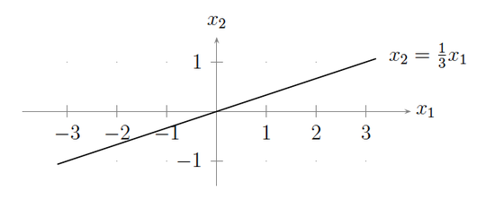
Example 1.2.3. Let us take the following system of one linear equation in the two unknowns \(x_1\) and \(x_2\):
\begin{equation*} x_1 - 3x_2 = 0. \end{equation*}
In this case, there are infinitely many solutions given by the set \(\{x_2 = \frac{1}{3}x_1 \mid x_1\in \mathbb{R}\}\). You can think of this solution set as a line in the Euclidean plane \(\mathbb{R}^{2}\):
In general, a system of \(m\) linear equations in \(n\) unknowns \(x_1,x_2,\ldots,x_n\) is a collection of equations of the form
\begin{equation} \label{eq:linear system} \left. \begin{array}{rl} a_{11} x_1 + a_{12} x_2 + \cdots + a_{1n} x_n &= b_1\\ a_{21} x_1 + a_{22} x_2 + \cdots + a_{2n} x_n &= b_2\\ \vdots \qquad \qquad & \vdots\\ a_{m1} x_1 + a_{m2} x_2 + \cdots + a_{mn} x_n &= b_m \end{array} \right\}, \tag{1.2.1} \end{equation}
where the \(a_{ij}\)'s are the coefficients (usually real or complex numbers) in front of the unknowns \(x_j\), and the \(b_i\)'s are also fixed real or complex numbers. A solution is a set of numbers \(s_1,s_2,\ldots,s_n\) such that, substituting \(x_1=s_1,x_2=s_2,\ldots,x_n=s_n\) for the unknowns, all of the equations in System 1.2.1 hold. Linear Algebra is a theory that concerns the solutions and the structure of solutions for linear equations. As this course progresses, you will see that there is a lot of subtlety in fully understanding the solutions for such equations.
1.3 Systems of linear equations
1.3.1 Linear equations
Before going on, let us reformulate the notion of a system of linear equations into the language of functions. This will also help us understand the adjective ``linear'' a bit better. A function \(f\) is a map
\begin{equation} f: X \to Y \tag{1.3.1} \end{equation}
from a set \(X\) to a set \(Y\). The set \(X\) is called the domain of the function, and the set \(Y\) is called the target space or codomain of the function. An equation is
\begin{equation} f(x)=y, \tag{1.3.2} \end{equation}
where \(x \in X\) and \(y \in Y\). (If you are not familiar with the abstract notions of sets and functions, then please consult Appendix A.)
Example 1.3.1. Let \(f:\mathbb{R}\to\mathbb{R}\) be the function \(f(x)=x^3-x\). Then \(f(x)=x^3-x=1\) is an equation. The domain and target space are both the set of real numbers \(\mathbb{R}\) in this case.
In this setting, a system of equations is just another kind of equation.
Example 1.3.2. Let \(X=Y=\mathbb{R}^2=\mathbb{R} \times \mathbb{R}\) be the Cartesian product of the set of real numbers. Then define the function \(f:\mathbb{R}^2 \to \mathbb{R}^2\) as
\begin{equation} f(x_1,x_2) = (2x_1+x_2, x_1-x_2), \tag{1.3.3} \end{equation}
and set \(y=(0,1)\). Then the equation \(f(x)=y\), where \(x=(x_1,x_2)\in \mathbb{R}^2\), describes the system of linear equations of Example 1.2.1.
The next question we need to answer is, ``what is a linear equation?'' Building on the definition of an equation, a linear equation is any equation defined by a ``linear'' function \(f\) that is defined on a ``linear'' space (a.k.a.~a vector space as defined in Section 4.1). We will elaborate on all of this in future lectures, but let us demonstrate the main features of a ``linear'' space in terms of the example \(\mathbb{R}^2\). Take \(x=(x_1,x_2), y=(y_1,y_2) \in \mathbb{R}^2\). There are two ``linear'' operations defined on \(\mathbb{R}^2\), namely addition and scalar multiplication:
\begin{align} x+y &: = (x_1+y_1, x_2+y_2) && \text{(vector addition)} \tag{1.3.4} \\ cx & := (cx_1,cx_2) && \text{(scalar multiplication).} \tag{1.3.5} \end{align}
A ``linear'' function on \(\mathbb{R}^{2}\) is then a function \(f\) that interacts with these operations in the following way:
\begin{align} f(cx) &= cf(x) \tag{1.3.6} \\ f(x+y) & = f(x) + f(y). \tag{1.3.7}\end{align}
You should check for yourself that the function \(f\) in Example 1.3.2 has these two properties.
1.3.2 Non-linear equations
(Systems of) Linear equations are a very important class of (systems of) equations. You will learn techniques in this class that can be used to solve any systems of linear equations. Non-linear equations, on the other hand, are significantly harder to solve. An example is a quadratic equation such as
\begin{equation} x^2 + x -2 =0, \tag{1.3.8} \end{equation}
which, for no completely obvious reason, has exactly two solutions \(x=-2\) and \(x=1\). Contrast this with the equation
\begin{equation} x^2 + x +2 =0, \tag{1.3.9} \end{equation}
which has no solutions within the set \(\mathbb{R}\) of real numbers. Instead, it is has two complex solutions \(\frac{1}{2}(-1\pm i\sqrt{7}) \in \mathbb{C}\), where \(i=\sqrt{-1}\). (Complex numbers are discussed in more detail in Chapter 2.) In general, recall that the quadratic equation \(x^2 +bx+c=0\) has the two solutions
\[ x = -\frac{b}{2} \pm \sqrt{\frac{b^2}{4}-c}.\]
1.3.3 Linear transformations
The set \(\mathbb{R}^2\) can be viewed as the Euclidean plane. In this context, linear functions of the form \(f:\mathbb{R}^2 \to \mathbb{R}\) or \(f:\mathbb{R}^2 \to \mathbb{R}^2\) can be interpreted geometrically as ``motions'' in the plane and are called linear transformations.
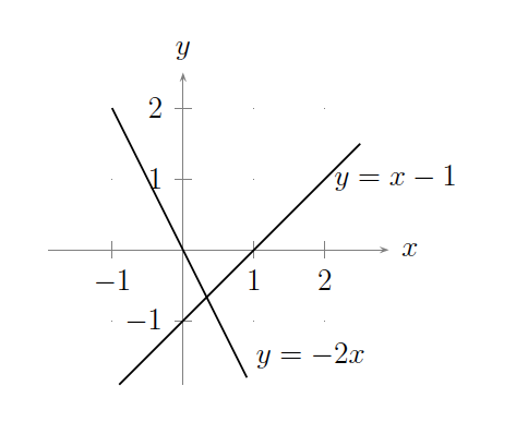
Example 1.3.3. Recall the following linear system from Example 1.2.1:
\begin{equation*} \left. \begin{array}{rl} 2x_1 + x_2 &= 0\\ x_1 - x_2 &= 1 \end{array} \right\}. \end{equation*}
Each equation can be interpreted as a straight line in the plane, with solutions \((x_1,x_2)\) to the linear system given by the set of all points that simultaneously lie on both lines. In this case, the two lines meet in only one location, which corresponds to the unique solution to the linear system as illustrated in the following figure:
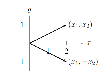
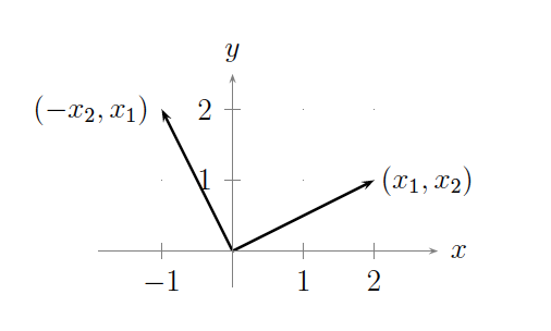
Example 1.3.4. The linear map \(f(x_1,x_2) = (x_1,-x_2)\) describes the ``motion'' of reflecting a vector across the \(x\)-axis, as illustrated in the following figure: Example 1.3.5. The linear map \(f(x_1,x_2) = (-x_2,x_1)\) describes the ``motion'' of rotating a vector by \(90^0\) counterclockwise, as illustrated in the following figure:This example can easily be generalized to rotation by any arbitrary angle using Lemma 2.3.2. In particular, when points in \(\mathbb{R}^{2}\) are viewed as complex numbers, then we can employ the so-called polar form for complex numbers in order to model the ``motion'' of rotation. (Cf. Proof-Writing Exercise 5 in Exercises for Chapter 2.)
1.3.4 Applications of linear equations
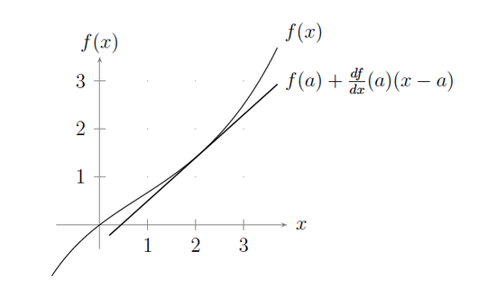
Linear equations pop up in many different contexts. For example, you can view the derivative \(\frac{df}{dx}(x)\) of a differentiable function \(f:\mathbb{R}\to\mathbb{R}\) as a linear approximation of \(f\). This becomes apparent when you look at the Taylor series of the function \(f(x)\) centered around the point \(x=a\) (as seen in a course like MAT 21C):
\begin{equation} f(x) = f(a) + \frac{df}{dx}(a) (x-a) + \cdots. \tag{1.3.10} \end{equation}
In particular, we can graph the linear part of the Taylor series versus the original function, as in the following figure:
Since \(f(a)\) and \(\frac{df}{dx}(a)\) are merely real numbers, \(f(a) + \frac{df}{dx}(a) (x-a)\) is a linear function in the single variable \(x\).
Similarly, if \(f:\mathbb{R}^n \to \mathbb{R}^m\) is a multivariate function, then one can still view the derivative of \(f\) as a form of a linear approximation for \(f\) (as seen in a course like MAT 21D).
What if there are infinitely many variables \(x_1, x_2,\ldots\)? In this case, the system of equations has the form
\begin{equation*} \left. \begin{array}{rl} a_{11} x_1 + a_{12} x_2 + \cdots &= y_1\\ a_{21} x_1 + a_{22} x_2 + \cdots &= y_2\\ \cdots & \end{array} \right\}. \end{equation*}
Hence, the sums in each equation are infinite, and so we would have to deal with infinite series. This, in particular, means that questions of convergence arise, where convergence depends upon the infinite sequence \(x=(x_1,x_2,\ldots)\) of variables. These questions will not occur in this course since we are only interested in finite systems of linear equations in a finite number of variables. Other subjects in which these questions do arise, though, include
- Differential Equations (as in a course like MAT 22B or MAT 118AB);
- Fourier Analysis (as in a course like MAT 129);
- Real and Complex Analysis (as in a course like MAT 125AB, MAT 185AB, MAT 201ABC, or MAT 202).
In courses like MAT 150ABC and MAT 250ABC, Linear Algebra is also seen to arise in the study of such things as symmetries, linear transformations, and Lie Algebra theory.
Contributors
- Isaiah Lankham, Mathematics Department at UC Davis
- Bruno Nachtergaele, Mathematics Department at UC Davis
- Anne Schilling, Mathematics Department at UC Davis
Both hardbound and softbound versions of this textbook are available online at WorldScientific.com.


