2.3: Polar Form and Geometric Interpretation

Last updated
Save as PDF

Page ID: 268

$ \newcommand{\vecs}[1]{\overset { \scriptstyle \rightharpoonup} {\mathbf{#1}} } $ $ \newcommand{\vecd}[1]{\overset{-\!-\!\rightharpoonup}{\vphantom{a}\smash {#1}}} $$\newcommand{\id}{\mathrm{id}}$ $ \newcommand{\Span}{\mathrm{span}}$ $ \newcommand{\kernel}{\mathrm{null}\,}$ $ \newcommand{\range}{\mathrm{range}\,}$ $ \newcommand{\RealPart}{\mathrm{Re}}$ $ \newcommand{\ImaginaryPart}{\mathrm{Im}}$ $ \newcommand{\Argument}{\mathrm{Arg}}$ $ \newcommand{\norm}[1]{\| #1 \|}$ $ \newcommand{\inner}[2]{\langle #1, #2 \rangle}$ $ \newcommand{\Span}{\mathrm{span}}$ $\newcommand{\id}{\mathrm{id}}$ $ \newcommand{\Span}{\mathrm{span}}$ $ \newcommand{\kernel}{\mathrm{null}\,}$ $ \newcommand{\range}{\mathrm{range}\,}$ $ \newcommand{\RealPart}{\mathrm{Re}}$ $ \newcommand{\ImaginaryPart}{\mathrm{Im}}$ $ \newcommand{\Argument}{\mathrm{Arg}}$ $ \newcommand{\norm}[1]{\| #1 \|}$ $ \newcommand{\inner}[2]{\langle #1, #2 \rangle}$ $ \newcommand{\Span}{\mathrm{span}}$$\newcommand{\AA}{\unicode[.8,0]{x212B}}$

As mentioned above, $\mathbb{C}$ coincides with the plane $\mathbb{R}^{2}$ when viewed as a set of ordered pairs of real numbers. Therefore, we can use polar coordinates as an alternate way to uniquely identify a complex number. This gives rise to the so-called polar form for a complex number, which often turns out to be a convenient representation for complex numbers.

Polar form for complex numbers

The following diagram summarizes the relations between Cartesian and polar coordinates in $\mathbb{R}^2$:

$Screen shot 2014-01-03 at 12.20.51 PM.png$

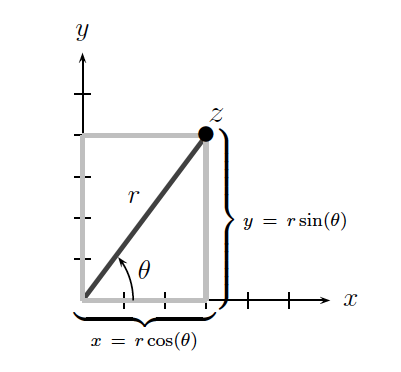
We call the ordered pair $(x, y)$ the rectangular coordinates for the complex number $z$.

We also call the ordered pair $(r, \theta)$ the polar coordinates for the complex number $z$. The radius $r = |z|$ is called the modulus of $z$ (as defined in Section 2.2.4 above), and the angle $\theta = \Argument(z)$ is called the argument of $z$. Since the argument of a complex number describes an angle that is measured relative to the $x$-axis, it is important to note that $\theta$ is only well-defined up to adding multiples of $2\pi$. As such, we restrict $\theta \in [0, 2\pi)$ and add or subtract multiples of $2\pi$ as needed (e.g., when multiplying two complex numbers so that their arguments are added together) in order to keep the argument within this range of values.

It is straightforward to transform polar coordinates into rectangular coordinates using the equations

\begin{equation} \label{eq:sincos}
x = r\cos(\theta)
{\rm \quad and \quad }
y = r\sin(\theta). \tag{2.3.1}
\end{equation}

In order to transform rectangular coordinates into polar coordinates, we first note that $r = \sqrt{x^{2} + y^{2}}$ is just the complex modulus. Then, $\theta$ must be chosen so that it satisfies the bounds $0 \leq \theta < 2\pi$ in addition to the simultaneous equations (2.3.1) where we are assuming that $z \neq 0$.

Summarizing:

\[ z = x + y i = r\cos(\theta) + r\sin(\theta)i = r(\cos(\theta) + \sin(\theta)i). \]

Part of the utility of this expression is that the size $r = |z|$ of $z$ is explicitly part of the very definition since it is easy to check that $|\cos(\theta) + \sin(\theta)i| = 1$ for any choice of $\theta \in \mathbb{R}$.

Closely related is the exponential form for complex numbers, which does nothing more than replace the expression $\cos(\theta) + \sin(\theta)i$ with $e^{i \theta}$. The real power of this definition is that this exponential notation turns out to be completely consistent with the usual usage of exponential notation for real numbers.

Example $\PageIndex{1}$:

The complex number $i$ in polar coordinates is expressed as $e^{i\pi/2}$, whereas the number $-1$ is given by $e^{i\pi}$.

2.3.2 Geometric multiplication for complex numbers

As discussed in Section 2.3.1 above, the general exponential form for a complex number $z$ is an expression of the form $r e^{i \theta}$ where $r$ is a non-negative real number and $\theta \in [0, 2\pi)$. The utility of this notation is immediately observed when multiplying two complex numbers:

Note

Lemma 2.3.2. Let $z_{1} = r_{1}e^{i \theta_{1}}, z_{2} = r_{2}e^{i \theta_{2}} \in \mathbb{C}$ be complex numbers in exponential form. Then

\[ z_1 z_2 = r_1 r_2 e^{i(\theta_1+\theta_2)}. \]

Proof.

By direct computation,

\begin{equation*}
\begin{split}
z_{1}z_{2} &= (r_{1}e^{i\theta_{1}})(r_{2}e^{i\theta_{2}})
= r_{1}r_{2}e^{i\theta_{1}} e^{i\theta_{2}} \\
&= r_1 r_2 (\cos\theta_1 +i \sin\theta_1) (\cos\theta_2+i\sin\theta_2)\\
&= r_1 r_2\bigl[ (\cos\theta_1 \cos\theta_2 -\sin\theta_1 \sin\theta_2)
+i (\sin\theta_1 \cos\theta_2 +\cos\theta_1\sin\theta_2) \bigr]\\
&= r_1 r_2 \bigl[ \cos(\theta_1+\theta_2) + i \sin(\theta_1+\theta_2) \bigr]
= r_1 r_2 e^{i(\theta_1+\theta_2)},
\end{split}
\end{equation*}

where we have used the usual formulas for the sine and cosine of the sum of two angles.

$\square$

In particular, Lemma 2.3.2 shows that the modulus $|z_{1}z_{2}|$ of the product is the product of the moduli $r_{1}$ and $r_{2}$ and that the argument $\Argument(z_{1}z_{2})$ of the product is the sum of the arguments $\theta_{1} + \theta_{2}$.

2.3.3 Exponentiation and root extraction

Another important use for the polar form of a complex number is in exponentiation. The simplest possible situation here involves the use of a positive integer as a power, in which case exponentiation is nothing more than repeated multiplication. Given the observations in Section 2.3.2 above and using some trigonometric identities, one quickly obtains the following fundamental result.

Theorem 2.3.3. Let $z = r(\cos(\theta) + \sin(\theta)i)$ be a complex number in polar form and $n \in \mathbb{Z}_{+}$ be a positive integer. Then

the exponentiation $z^{n} = r^{n}(\cos(n\theta) + \sin(n\theta)i)$ and
the $n^{\rm th}$ roots of $z$ are given by the $n$ complex numbers

\[
z_{k} = r^{1/n}\left[\cos\left(\frac{\theta}{n} +
\frac{2\pi k}{n}\right) + \sin\left(\frac{\theta}{n} +
\frac{2\pi k}{n}\right)i\right]
= r^{1/n} e^{\frac{i}{n}(\theta + 2\pi k)},
\]

where $k = 0, 1, 2, \ldots, n - 1$.

Note, in particular, that we are not only always guaranteed the existence of an $n^{\rm th}$ root for any complex number, but that we are also always guaranteed to have exactly $n$ of them. This level of completeness in root extraction contrasts very sharply with the delicate care that must be taken when one wishes to extract roots of real numbers without the aid of complex numbers.

An important special case of de Moivre's Formula yields an infinite family of well-studied numbers called the roots of unity. By unity, we just mean the complex number $1 = 1 + 0i$, and by the $n^{\rm th}$ roots of unity, we mean the $n$ numbers

\begin{align*}
z_{k}
\ = \ &
1^{1/n}\left[\cos\left(\frac{0}{n} +
\frac{2\pi k}{n}\right) + \sin\left(\frac{0}{n} +
\frac{2\pi k}{n}\right)i\right]
\\
\ =\ &
\cos\left(\frac{2\pi
k}{n}\right) + \sin\left(\frac{2\pi
k}{n}\right)i\\
\ =\ & e^{2\pi i (k/n)},
\end{align*}
where $k = 0, 1, 2, \ldots, n - 1$. These numbers have many interesting properties and important applications despite how simple they might appear to be.

Example $\PageIndex{4}$

To find all solutions of the equation $z^3+8=0$ for $z\in \mathbb{C}$, we may write $z=r e^{i\theta}$ in polar form with $r>0$ and $\theta\in[0,2\pi)$. Then the equation $z^3+8=0$ becomes $z^3=r^3 e^{i 3\theta}=-8=8 e^{i\pi}$ so that $r=2$ and $3\theta=\pi+2\pi k$ for $k=0,1,2$. This means that there are three distinct solutions when $\theta \in [0,2\pi)$, namely $\theta=\frac{\pi}{3}$, $\theta=\pi$, and $\theta=\frac{5\pi}{3}$.

2.3.4 Some complex elementary functions

We conclude these notes by defining three of the basic elementary functions that take complex arguments. In this context, ``elementary function'' is used as a technical term and essentially means something like ``one of the most common forms of functions encountered when beginning to learn Calculus.'' The most basic elementary functions include the familiar polynomial and algebraic functions, such as the $n^{\rm th}$ root function, in addition to the somewhat more sophisticated exponential function, the trigonometric functions, and the logarithmic function. For the purposes of these notes, we will now define the complex exponential function and two complex trigonometric functions. Definitions for the remaining basic elementary functions can be found in any book on Complex Analysis.

The basic groundwork for defining the complex exponential function was already put into place in Sections 2.3.1 and 2.3.2 above. In particular, we have already defined the expression $e^{i\theta}$ to mean the sum $\cos(\theta) + \sin(\theta)i$ for any real number $\theta$. Historically, this equivalence is a special case of the more general Euler's formula:

\[ e^{x + y i} = e^{x}(\cos(y) + \sin(y)i), \]

which we here take as our definition of the complex exponential function applied to any complex number $x + y i$ for $x, y \in \mathbb{R}$.

Given this exponential function, one can then define the complex sine function and the complex cosine function as

\[ \sin(z) = \frac{e^{i z} - e^{-i z}}{2 i} {\rm \quad and \quad} \cos(z) = \frac{e^{i z} + e^{-i z}}{2}.\]

Remarkably, these functions retain many of their familiar properties, which should be taken as a sign that the definitions --- however abstract --- have been well thought-out. We summarize a few of these properties as follows.

Theorem 2.3.5

Given $z_{1}, z_{2} \in \mathbb{C}$,

$e^{z_{1} + z_{2}} = e^{z_{1}} e^{z_{2}}$ and $e^{z} \neq 0 $ for any choice of $z \in \mathbb{C}$.
$\sin^{2}(z_{1}) + \cos^{2}(z_{1}) = 1$.
$\sin(z_{1} + z_{2}) = \sin(z_{1})\cdot\cos(z_{2}) + \cos(z_{1})\cdot\sin(z_{2})$.
$\cos(z_{1} + z_{2}) = \cos(z_{1})\cdot\cos(z_{2}) - \sin(z_{1})\cdot\sin(z_{2})$.

Contributors

Both hardbound and softbound versions of this textbook are available online at WorldScientific.com.