5.2: Properties of Linear Transformations

Learning Objectives

• T/F: Translating the Cartesian plane \(2\) units up is a linear transformation.
• T/F: If \(T\) is a linear transformation, then \(T(\vec{0})=\vec{0}\).

In the previous section we discussed standard transformations of the Cartesian plane – rotations, reflections, etc. As a motivational example for this section’s study, let’s consider another transformation – let’s find the matrix that moves the unit square one unit to the right (see Figure \(\PageIndex{1}\)). This is called a translation.

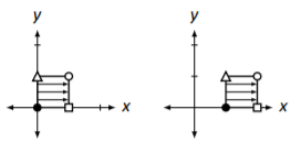
Figure \(\PageIndex{1}\): Translating the unit square one unit to the right.

Our work from the previous section allows us to find the matrix quickly. By looking at the picture, it is easy to see that \(\vec{e_{1}}\) is moved to \(\left[\begin{array}{c}{2}\\{0}\end{array}\right]\) and \(\vec{e_{2}}\) is moved to \(\left[\begin{array}{c}{1}\\{1}\end{array}\right]\). Therefore, the transformation matrix should be

\[A=\left[\begin{array}{cc}{2}&{1}\\{0}&{1}\end{array}\right].\nonumber \]

However, look at Figure \(\PageIndex{2}\) where the unit square is drawn after being transformed by \(A\). It is clear that we did not get the desired result; the unit square was not translated, but rather stretched/sheared in some way.

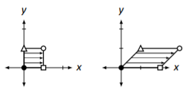
Figure \(\PageIndex{2}\): Actual transformation of the unit square by matrix \(A\).

What did we do wrong? We will answer this question, but first we need to develop a few thoughts and vocabulary terms.

We’ve been using the term “transformation” to describe how we’ve changed vectors. In fact, “transformation” is synonymous to “function.” We are used to functions like \(f(x) = x^2\), where the input is a number and the output is another number. In the previous section, we learned about transformations (functions) where the input was a vector and the output was another vector. If \(A\) is a “transformation matrix,” then we could create a function of the form \(T(\vec{x})=A\vec{x}\). That is, a vector \(\vec{x}\) is the input, and the output is \(\vec{x}\) multiplied by \(A\).\(^{1}\)

When we defined \(f(x) = x^2\) above, we let the reader assume that the input was indeed a number. If we wanted to be complete, we should have stated \[f:\mathbb{R} \to\mathbb{R} \quad \text{ where } \quad f(x)=x^2.\nonumber \] The first part of that line told us that the input was a real number (that was the first \(\mathbb{R}\)) and the output was also a real number (the second \(\mathbb{R}\)).

To define a transformation where a 2D vector is transformed into another 2D vector via multiplication by a \(2\times 2\) matrix \(A\), we should write

\[T:\mathbb{R}^{2}\to\mathbb{R}^{2}\quad\text{where}\quad T(\vec{x})=A\vec{x}.\nonumber \]

Here, the first \(\mathbb{R}^{2}\) means that we are using 2D vectors as our input, and the second \(\mathbb{R}^{2}\) means that a 2D vector is the output.

Consider a quick example:

\[T:\mathbb{R}^{2}\to\mathbb{R}^{3}\quad\text{where}\quad T\left(\left[\begin{array}{c}{x_{1}}\\{x_{2}}\end{array}\right]\right)=\left[\begin{array}{c}{x_{1}^{2}}\\{2x_{1}}\\{x_{1}x_{2}}\end{array}\right].\nonumber \]

Notice that this takes 2D vectors as input and returns 3D vectors as output. For instance,

\[T\left(\left[\begin{array}{c}{3}\\{-2}\end{array}\right]\right)=\left[\begin{array}{c}{9}\\{6}\\{-6}\end{array}\right].\nonumber \]

We now define a special type of transformation (function).

Definition: Linear Transformation

A transformation \(T:\mathbb{R}^{n}\to\mathbb{R}^{m}\) is a linear transformation if it satisfies the following two properties:

1. \(T(\vec{x}+\vec{y})=T(\vec{x})+T(\vec{y})\) for all vectors \(\vec{x}\) and \(\vec{y}\), and
2. \(T(k\vec{x})=kT(\vec{x})\) for all vectors \(\vec{x}\) and all scalars \(k\).

If \(T\) is a linear transformation, it is often said that “\(T\) is linear.”

Let’s learn about this definition through some examples.

Example \(\PageIndex{1}\)

Determine whether or not the transformation \(T:\mathbb{R}^{2}\to\mathbb{R}^{3}\) is a linear transformation, where

\[T\left(\left[\begin{array}{c}{x_{1}}\\{x_{2}}\end{array}\right]\right)=\left[\begin{array}{c}{x_{1}^{2}}\\{2x_{1}}\\{x_{1}x_{2}}\end{array}\right].\nonumber \]

Solution

We’ll arbitrarily pick two vectors \(\vec{x}\) and \(\vec{y}\):

\[\vec{x}=\left[\begin{array}{c}{3}\\{-2}\end{array}\right]\quad\text{and}\quad\vec{y}=\left[\begin{array}{c}{1}\\{5}\end{array}\right].\nonumber \]

Let’s check to see if \(T\) is linear by using the definition.

1. Is \(T(\vec{x}+\vec{y}) = T(\vec{x})+T(\vec{y})\)? First, compute \(\vec{x}+\vec{y}\):
   \[\vec{x}+\vec{y}=\left[\begin{array}{c}{3}\\{-2}\end{array}\right]+\left[\begin{array}{c}{1}\\{5}\end{array}\right]=\left[\begin{array}{c}{4}\\{3}\end{array}\right].\nonumber \]
   Now compute \(T(\vec{x})\), \(T(\vec{y})\), and \(T(\vec{x}+\vec{y})\):

\[\begin{array}{ccccc}{\begin{aligned}T(\vec{x})&=T\left(\left[\begin{array}{c}{3}\\{-2}\end{array}\right]\right) \\ &=\left[\begin{array}{c}{9}\\{6}\\{-6}\end{array}\right]\end{aligned}}&{\quad}&{\begin{aligned}T(\vec{y})&=T\left(\left[\begin{array}{c}{1}\\{5}\end{array}\right]\right) \\ &=\left[\begin{array}{c}{1}\\{2}\\{5}\end{array}\right]\end{aligned}}&{\quad}&{\begin{aligned}T(\vec{x}+\vec{y})&=T\left(\left[\begin{array}{c}{4}\\{3}\end{array}\right]\right) \\ &=\left[\begin{array}{c}{16}\\{8}\\{12}\end{array}\right]\end{aligned}}\end{array}\nonumber \]

Is \(T(\vec{x}+\vec{y}) = T(\vec{x})+T(\vec{y})\)?

\[\left[\begin{array}{c}{9}\\{6}\\{-6}\end{array}\right]+\left[\begin{array}{c}{1}\\{2}\\{5}\end{array}\right]\stackrel{!}{\neq} \left[\begin{array}{c}{16}\\{8}\\{12}\end{array}\right].\nonumber \]

Therefore, \(T\) is not a linear transformation.

So we have an example of something that doesn’t work. Let’s try an example where things do work.\(^{2}\)

Example \(\PageIndex{2}\)

Determine whether or not the transformation \(T\) : \(\mathbb{R}^{2}\to\mathbb{R}^{2}\) is a linear transformation, where \(T(\vec{x})=A\vec{x}\) and

\[A=\left[\begin{array}{cc}{1}&{2}\\{3}&{4}\end{array}\right].\nonumber \]

Solution

Let’s start by again considering arbitrary \(\vec{x}\) and \(\vec{y}\). Let’s choose the same \(\vec{x}\) and \(\vec{y}\) from Example \(\PageIndex{1}\).

\[\vec{x}=\left[\begin{array}{c}{3}\\{-2}\end{array}\right]\quad\text{and}\quad\vec{y}=\left[\begin{array}{c}{1}\\{5}\end{array}\right].\nonumber \]

If the lineararity properties hold for these vectors, then maybe it is actually linear (and we’ll do more work).

1. Is \(T(\vec{x}+\vec{y}) = T(\vec{x})+T(\vec{y})\)? Recall:
   \[\vec{x}+\vec{y}=\left[\begin{array}{c}{4}\\{3}\end{array}\right].\nonumber \]
   Now compute \(T(\vec{x})\), \(T(\vec{y})\), and \(T(\vec{x})+T(\vec{y})\):
   \[\begin{array}{ccccc}{\begin{aligned}T(\vec{x})&=T\left(\left[\begin{array}{c}{3}\\{-2}\end{array}\right]\right) \\ &=\left[\begin{array}{c}{-1}\\{1}\end{array}\right]\end{aligned}}&{\quad}&{\begin{aligned}T(\vec{y})&=T\left(\left[\begin{array}{c}{1}\\{5}\end{array}\right]\right) \\ &=\left[\begin{array}{c}{11}\\{23}\end{array}\right]\end{aligned}}&{\quad}&{\begin{aligned}T(\vec{x}+\vec{y})&=T\left(\left[\begin{array}{c}{4}\\{3}\end{array}\right]\right) \\ &=\left[\begin{array}{c}{10}\\{24}\end{array}\right]\end{aligned}}\end{array}\nonumber \]
   Is \(T(\vec{x}+\vec{y})=T(\vec{x})+T(\vec{y})\).
   \[\left[\begin{array}{c}{-1}\\{1}\end{array}\right]+\left[\begin{array}{c}{11}\\{23}\end{array}\right]\stackrel{!}{=}\left[\begin{array}{c}{10}\\{24}\end{array}\right].\nonumber \]
   So far, so good: \(T(\vec{x}+\vec{y})\) is equal to \(T(\vec{x})+T(\vec{y})\).
2. Is \(T(k\vec{x}) = kT(\vec{x})\)? Let’s arbitrarily pick \(k=7\), and use \(\vec{x}\) as before.
   \[\begin{align*}\begin{aligned}T(7\vec{x})&=T\left(\left[\begin{array}{c}{21}\\{-14}\end{array}\right]\right) \\ &=\left[\begin{array}{c}{-7}\\{7}\end{array}\right] \\ &=7\left[\begin{array}{c}{-1}\\{1}\end{array}\right] \\ &=7\cdot T(\vec{x}) !\end{aligned}\end{align*}\nonumber \]
   So far it seems that \(T\) is indeed linear, for it worked in one example with arbitrarily chosen vectors and scalar. Now we need to try to show it is always true.
   Consider \(T(\vec{x}+\vec{y})\). By the definition of \(T\), we have
   \[T(\vec{x}+\vec{y}) = A(\vec{x}+\vec{y}).\nonumber \]
   By Theorem 2.2.1, part 2 we state that the Distributive Property holds for matrix multiplication.\(^{3}\) So \(A(\vec{x}+\vec{y}) = A\vec{x} +A\vec{y}\). Recognize now that this last part is just \(T(\vec{x}) + T(\vec{y})\)! We repeat the above steps, all together:
   \[\begin{align*}\begin{aligned}T(\vec{x}+\vec{y})&=A(\vec{x}+\vec{y}) &\text{(by the definition of }T\text{ in this example)} \\ &=A\vec{x}+A\vec{y}&\text{(by the Distributive Property)} \\ &=T(\vec{x})+T(\vec{y}) &\text{(again, by the definition of }T\text{)}\end{aligned}\end{align*}\nonumber \]
   Therefore, no matter what \(\vec{x}\) and \(\vec{y}\) are chosen, \(T(\vec{x}+\vec{y}) = T(\vec{x}) + T(\vec{y})\). Thus the first part of the linearity definition is satisfied.
   The second part is satisfied in a similar fashion. Let \(k\) be a scalar, and consider:
   \[\begin{align*}\begin{aligned}T(k\vec{x})&=A(k\vec{x}) &\text{(by the definition of }T\text{ is this example)} \\ &=kA\vec{x} &\text{(by Theorem 2.2.1 part 3)} \\ &=kT(\vec{x}) &\text{(again, by the definition of }T\text{)}\end{aligned}\end{align*}\nonumber \]
   Since \(T\) satisfies both parts of the definition, we conclude that \(T\) is a linear transformation.

We have seen two examples of transformations so far, one which was not linear and one that was. One might wonder “Why is linearity important?”, which we’ll address shortly.

First, consider how we proved the transformation in Example \(\PageIndex{2}\) was linear. We defined \(T\) by matrix multiplication, that is, \(T(\vec{x}) = A\vec{x}\). We proved \(T\) was linear using properties of matrix multiplication – we never considered the specific values of \(A\)! That is, we didn’t just choose a good matrix for \(T\); any matrix \(A\) would have worked. This leads us to an important theorem. The first part we have essentially just proved; the second part we won’t prove, although its truth is very powerful.

Theorem \(\PageIndex{1}\): Matrices and Linear Transformations

1. Define \(T\): \(\mathbb{R}^{n}\to\mathbb{R}^{m}\) by \(T(\vec{x})=A\vec{x}\), where \(A\) is an \(m\times n\) matrix. Then \(T\) is a linear transformation.
2. Let \(T\): \(\mathbb{R}^{n}\to\mathbb{R}^{m}\) be any linear transformation. Then there exists an unique \(m\times n\) matrix \(A\) such that \(T(\vec{x})=A\vec{x}\).

The second part of the theorem says that all linear transformations can be described using matrix multiplication. Given any linear transformation, there is a matrix that completely defines that transformation. This important matrix gets its own name.

Definition: Standard Matrix of a Linear Transformation

Let \(T\): \(\mathbb{R}^{n}\to\mathbb{R}^{m}\) be a linear transformaton. By Theorem \(\PageIndex{1}\), there is a matrix \(A\) such that \(T(\vec{x})=A\vec{x}\). This matrix \(A\) is called the standard matrix of the linear transformation \(T\), and is denoted \([ T ]\).\(^{a}\)

\(\rule{5cm}{0.4pt}\)

[a] The matrix–like brackets around \(T\) suggest that the standard matrix \(A\) is a matrix “with \(T\) inside.”

While exploring all of the ramifications of Theorem \(\PageIndex{1}\) is outside the scope of this text, let it suffice to say that since 1) linear transformations are very, very important in economics, science, engineering and mathematics, and 2) the theory of matrices is well developed and easy to implement by hand and on computers, then 3) it is great news that these two concepts go hand in hand.

We have already used the second part of this theorem in a small way. In the previous section we looked at transformations graphically and found the matrices that produced them. At the time, we didn’t realize that these transformations were linear, but indeed they were.

This brings us back to the motivating example with which we started this section. We tried to find the matrix that translated the unit square one unit to the right. Our attempt failed, and we have yet to determine why. Given our link between matrices and linear transformations, the answer is likely “the translation transformation is not a linear transformation.” While that is a true statement, it doesn’t really explain things all that well. Is there some way we could have recognized that this transformation wasn’t linear?\(^{4}\)

Yes, there is. Consider the second part of the linear transformation definition. It states that \(T(k\vec{x}) = kT(\vec{x})\) for all scalars \(k\). If we let \(k=0\), we have \(T(0\vec{x}) = 0\cdot T(\vec{x})\), or more simply, \(T(\vec{0}) =\vec{0}\). That is, if \(T\) is to be a linear transformation, it must send the zero vector to the zero vector.

This is a quick way to see that the translation transformation fails to be linear. By shifting the unit square to the right one unit, the corner at the point \((0,0)\) was sent to the point \((1,0)\), i.e.,

\[\text{the vector }\left[\begin{array}{c}{0}\\{0}\end{array}\right]\text{ was sent to the vector }\left[\begin{array}{c}{1}\\{0}\end{array}\right].\nonumber \]

This property relating to \(\vec{0}\) is important, so we highlight it here.

Key Idea \(\PageIndex{1}\): Linear Transformations and \(\vec{0}\)

Let \(T\): \(\mathbb{R}^{n}\to\mathbb{R}^{m}\) be a linear transformation. Then:

\[T(\vec{0_{n}})=\vec{0_{m}}.\nonumber \]

That is, the zero vector in \(\mathbb{R}^{n}\) gets sent to the zero vector in \(\mathbb{R}^{m}\).

The interested reader may wish to read the footnote below.\(^{5}\)

The Standard Matrix of a Linear Transformation

It is often the case that while one can describe a linear transformation, one doesn’t know what matrix performs that transformation (i.e., one doesn’t know the standard matrix of that linear transformation). How do we systematically find it? We’ll need a new definition.

Definition: Standad Unit Vectors

In \(\mathbb{R}^{n}\), the standard unit vectors \(\vec{e_{i}}\) are the vectors with a \(1\) in the \(i^{\text{th}}\) entry and \(0\)s everywhere else.

We’ve already seen these vectors in the previous section. In \(\mathbb{R}^{2}\), we identified

\[\vec{e_{1}}=\left[\begin{array}{c}{1}\\{0}\end{array}\right]\quad\text{and}\quad\vec{e_{2}}=\left[\begin{array}{c}{0}\\{1}\end{array}\right].\nonumber \]

In \(\mathbb{R}^{4}\), there are \(4\) standard unit vectors:

\[\vec{e_{1}}=\left[\begin{array}{c}{1}\\{0}\\{0}\\{0}\end{array}\right],\quad\vec{e_{2}}=\left[\begin{array}{c}{0}\\{1}\\{0}\\{0}\end{array}\right],\quad\vec{e_{3}}=\left[\begin{array}{c}{0}\\{0}\\{1}\\{0}\end{array}\right],\quad\text{and}\quad\vec{e_{4}}=\left[\begin{array}{c}{0}\\{0}\\{0}\\{1}\end{array}\right].\nonumber \]

How do these vectors help us find the standard matrix of a linear transformation? Recall again our work in the previous section. There, we practiced looking at the transformed unit square and deducing the standard transformation matrix \(A\). We did this by making the first column of \(A\) the vector where \(\vec{e_{1}}\) ended up and making the second column of \(A\) the vector where \(\vec{e_{2}}\) ended up. One could represent this with:

\[A=[T(\vec{e_{1}})\:\: T(\vec{e_{2}})]=[T].\nonumber \]

That is, \(T(\vec{e_{1}})\) is the vector where \(\vec{e_{1}}\) ends up, and \(T(\vec{e_{2}})\) is the vector where \(\vec{e_{2}}\) ends up.

The same holds true in general. Given a linear transformation \(T:\mathbb{R}^{n}\to\mathbb{R}^{m}\), the standard matrix of \(T\) is the matrix whose \(i^\text{th}\) column is the vector where \(\vec{e_{i}}\) ends up. While we won’t prove this is true, it is, and it is very useful. Therefore we’ll state it again as a theorem.

Theorem \(\PageIndex{2}\)

The Standard Matrix of a Linear Transformation

Let \(T\): \(\mathbb{R}^{n}\to\mathbb{R}^{m}\) be a linear transformation. Then \([T]\) is the \(m\times n\) matrix:

\[[T]=[T(\vec{e_{1}})\:\:T(\vec{e_{2}})\:\cdots\: T(\vec{e_{n}})].\nonumber \]

Let’s practice this theorem in an example.

Example \(\PageIndex{3}\)

Define \(T\): \(\mathbb{R}^{3}\to\mathbb{R}^{4}\) to be the linear transformation where

\[T\left(\left[\begin{array}{c}{x_{1}}\\{x_{2}}\\{x_{3}}\end{array}\right]\right)=\left[\begin{array}{c}{x_{1}+x_{2}}\\{3x_{1}-x_{3}}\\{2x_{2}+5x_{3}}\\{4x_{1}+3x_{2}+2x_{3}}\end{array}\right].\nonumber \]

Find \([T]\).

Solution

\(T\) takes vectors from \(\mathbb{R}^{3}\) into \(\mathbb{R}^{4}\), so \([\, T \, ]\) is going to be a \(4\times 3\) matrix. Note that

\[\vec{e_{1}}=\left[\begin{array}{c}{1}\\{0}\\{0}\end{array}\right],\quad\vec{e_{2}}=\left[\begin{array}{c}{0}\\{1}\\{0}\end{array}\right]\quad\text{and}\quad\vec{e_{3}}=\left[\begin{array}{c}{0}\\{0}\\{1}\end{array}\right].\nonumber \]

We find the columns of \([T]\) by finding where \(\vec{e_{1}}\), \(\vec{e_{2}}\) and \(\vec{e_{3}}\) are sent, that is, we find \(T(\vec{e_{1}})\), \(T(\vec{e_{2}})\) and \(T(\vec{e_{3}})\).

\[\begin{array}{ccccc}{\begin{aligned}T(\vec{e_{1}})&=T\left(\left[\begin{array}{c}{1}\\{0}\\{0}\end{array}\right]\right) \\ &=\left[\begin{array}{c}{1}\\{3}\\{0}\\{4}\end{array}\right]\end{aligned}}&{\quad}&{\begin{aligned}T(\vec{e_{2}})&=T\left(\left[\begin{array}{c}{0}\\{1}\\{0}\end{array}\right]\right) \\ &=\left[\begin{array}{c}{1}\\{0}\\{2}\\{3}\end{array}\right]\end{aligned}}&{\quad}&{\begin{aligned}T(\vec{e_{3}})&=T\left(\left[\begin{array}{c}{0}\\{0}\\{1}\end{array}\right]\right) \\ &=\left[\begin{array}{c}{0}\\{-1}\\{5}\\{2}\end{array}\right]\end{aligned}}\end{array}\nonumber \]

Thus

\[[T]=A=\left[\begin{array}{ccc}{1}&{1}&{0}\\{3}&{0}&{-1}\\{0}&{2}&{5}\\{4}&{3}&{2}\end{array}\right].\nonumber \]

Let’s check this. Consider the vector

\[\vec{x}=\left[\begin{array}{c}{1}\\{2}\\{3}\end{array}\right].\nonumber \]

Strictly from the original definition, we can compute that

\[T(\vec{x})=T\left(\left[\begin{array}{c}{1}\\{2}\\{3}\end{array}\right]\right)=\left[\begin{array}{c}{1+2}\\{3-3}\\{4+15}\\{4+6+6}\end{array}\right]=\left[\begin{array}{c}{3}\\{0}\\{19}\\{16}\end{array}\right].\nonumber \]

Now compute \(T(\vec{x})\) by computing \([T]\vec{x}=A\vec{x}\).

\[A\vec{x}=\left[\begin{array}{ccc}{1}&{1}&{0}\\{3}&{0}&{-1}\\{0}&{2}&{5}\\{4}&{3}&{2}\end{array}\right]\left[\begin{array}{c}{1}\\{2}\\{3}\end{array}\right]=\left[\begin{array}{c}{3}\\{0}\\{19}\\{16}\end{array}\right].\nonumber \]

They match!\(^{6}\)

Let’s do another example, one that is more application oriented.

Example \(\PageIndex{4}\)

A baseball team manager has collected basic data concerning his hitters. He has the number of singles, doubles, triples, and home runs they have hit over the past year. For each player, he wants two more pieces of information: the total number of hits and the total number of bases.

Using the techniques developed in this section, devise a method for the manager to accomplish his goal.

Solution

If the manager only wants to compute this for a few players, then he could do it by hand fairly easily. After all:

\[\text{total # hits = # of singles + # of doubles + # of triples + # of home runs,}\nonumber \]

and

\[\text{total # bases = # of singles + }2\times\text{# of doubles + }3\times\text{# of triples + }4\times\text{# of home runs.}\nonumber \]

However, if he has a lot of players to do this for, he would likely want a way to automate the work. One way of approaching the problem starts with recognizing that he wants to input four numbers into a function (i.e., the number of singles, doubles, etc.) and he wants two numbers as output (i.e., number of hits and bases). Thus he wants a transformation \(T\): \(\mathbb{R}^{4}\to\mathbb{R}^{2}\) where each vector in \(\mathbb{R}^{4}\) can be interpreted as

\[\left[\begin{array}{c}{\text{# of singles}} \\ {\text{# of doubles}} \\ {\text{# of triples}} \\ {\text{# of home runs}}\end{array}\right],\nonumber \]

and each vector in \(\mathbb{R}^{2}\) can be interpreted as

\[\left[\begin{array}{c}{\text{# of hits}} \\ {\text{# of bases}} \end{array}\right].\nonumber \]

To find \([T]\), he computes \(T(\vec{e_{1}})\), \(T(\vec{e_{2}})\), \(T(\vec{e_{3}})\) and \(T(\vec{e_{4}})\).

\[\begin{array}{ccc}{\begin{aligned}T(\vec{e_{1}})&=T\left(\left[\begin{array}{c}{1}\\{0}\\{0}\\{0}\end{array}\right]\right) \\ &=\left[\begin{array}{c}{1}\\{1}\end{array}\right]\end{aligned}}&{\quad}&{\begin{aligned}T(\vec{e_{2}})&=T\left(\left[\begin{array}{c}{0}\\{1}\\{0}\\{0}\end{array}\right]\right) \\ &=\left[\begin{array}{c}{1}\\{2}\end{array}\right]\end{aligned}}\\ {\begin{aligned}T(\vec{e_{3}})&=T\left(\left[\begin{array}{c}{0}\\{0}\\{1}\\{0}\end{array}\right]\right) \\ &=\left[\begin{array}{c}{1}\\{3}\end{array}\right]\end{aligned}}&{\quad}&{\begin{aligned}T(\vec{e_{4}})&=T\left(\left[\begin{array}{c}{0}\\{0}\\{0}\\{1}\end{array}\right]\right) \\ &=\left[\begin{array}{c}{1}\\{4}\end{array}\right]\end{aligned}} \end{array}\nonumber \]

(What do these calculations mean? For example, finding \(T(\vec{e_{3}}) = \left[\begin{array}{c}{1}\\{3}\end{array}\right]\) means that one triple counts as \(1\) hit and \(3\) bases.)
Thus our transformation matrix \([T]\) is

\[[T]=A=\left[\begin{array}{cccc}{1}&{1}&{1}&{1}\\{1}&{2}&{3}&{4}\end{array}\right].\nonumber \]

As an example, consider a player who had \(102\) singles, \(30\) doubles, \(8\) triples and \(14\) home runs. By using \(A\), we find that

\[\left[\begin{array}{cccc}{1}&{1}&{1}&{1}\\{1}&{2}&{3}&{4}\end{array}\right]\left[\begin{array}{c}{102}\\{30}\\{8}\\{14}\end{array}\right]=\left[\begin{array}{c}{154}\\{242}\end{array}\right],\nonumber \]

meaning the player had \(154\) hits and \(242\) total bases.

A question that we should ask concerning the previous example is “How do we know that the function the manager used was actually a linear transformation? After all, we were wrong before – the translation example at the beginning of this section had us fooled at first.”

This is a good point; the answer is fairly easy. Recall from Example \(\PageIndex{1}\) the transformation

\[T_{98}\left(\left[\begin{array}{c}{x_{1}}\\{x_{2}}\end{array}\right]\right)=\left[\begin{array}{c}{x_{1}^{2}}\\{2x_{1}}\\{x_{1}x_{2}}\end{array}\right]\nonumber \]

and from Example \(\PageIndex{3}\)

\[T_{100}\left(\left[\begin{array}{c}{x_{1}}\\{x_{2}}\\{x_{3}}\end{array}\right]\right)=\left[\begin{array}{c}{x_{1}+x_{2}}\\{3x_{1}-x_{3}}\\{2x_{2}+5x_{3}}\\{4x_{1}+3x_{2}+2x_{3}}\end{array}\right],\nonumber \]

where we use the subscripts for \(T\) to remind us which example they came from.

We found that \(T_{98}\) was not a linear transformation, but stated that \(T_{100}\) was (although we didn’t prove this). What made the difference?

Look at the entries of \(T_{98}(\vec{x})\) and \(T_{100}(\vec{x})\). \(T_{98}\) contains entries where a variable is squared and where \(2\) variables are multiplied together – these prevent \(T_{98}\) from being linear. On the other hand, the entries of \(T_{100}\) are all of the form \(a_1x_1 + \cdots + a_nx_n\); that is, they are just sums of the variables multiplied by coefficients. \(T\) is linear if and only if the entries of \(T(\vec{x})\) are of this form. (Hence linear transformations are related to linear equations, as defined in Section 1.1.) This idea is important.

Key Idea \(\PageIndex{2}\): Conditions on Linear Transformations

Let \(T\): \(\mathbb{R}^{n}\to\mathbb{R}^{m}\) be a transformation and consider the entries of

\[T(\vec{x})=T\left(\left[\begin{array}{c}{x_{1}}\\{x_{2}}\\{\vdots}\\{x_{n}}\end{array}\right]\right).\nonumber \]

\(T\) is linear if and only if each entry of \(T(\vec{x})\) is of the form \(a_{1}x_{1}+a_{2}x_{2}+\cdots a_{n}x_{n}.\)

Going back to our baseball example, the manager could have defined his transformation as

\[T\left(\left[\begin{array}{c}{x_{1}}\\{x_{2}}\\{x_{3}}\\{x_{4}}\end{array}\right]\right)=\left[\begin{array}{c}{x_{1}+x_{2}+x_{3}+x_{4}}\\{x_{1}+2x_{2}+3x_{3}+4x_{4}}\end{array}\right].\nonumber \]

Since that fits the model shown in Key Idea \(\PageIndex{2}\), the transformation \(T\) is indeed linear and hence we can find a matrix \([T]\) that represents it.

Let’s practice this concept further in an example.

Example \(\PageIndex{5}\)

Using Key Idea \(\PageIndex{2}\), determine whether or not each of the following transformations is linear.

\[T_{1}\left(\left[\begin{array}{c}{x_{1}}\\{x_{2}}\end{array}\right]\right)=\left[\begin{array}{c}{x_{1}+1}\\{x_{2}}\end{array}\right]\qquad T_{2}\left(\left[\begin{array}{c}{x_{1}}\\{x_{2}}\end{array}\right]\right)=\left[\begin{array}{c}{x_{1}/x_{2}}\\{\sqrt{x_{2}}}\end{array}\right] \qquad T_{3}\left(\left[\begin{array}{c}{x_{1}}\\{x_{2}}\end{array}\right]\right)=\left[\begin{array}{c}{\sqrt{7}x_{1}-x_{2}}\\{\pi x_{2}}\end{array}\right]\nonumber \]

Solution

\(T_1\) is not linear! This may come as a surprise, but we are not allowed to add constants to the variables. By thinking about this, we can see that this transformation is trying to accomplish the translation that got us started in this section – it adds \(1\) to all the \(x\) values and leaves the \(y\) values alone, shifting everything to the right one unit. However, this is not linear; again, notice how \(\vec{0}\) does not get mapped to \(\vec{0}\).

\(T_2\) is also not linear. We cannot divide variables, nor can we put variables inside the square root function (among other other things; again, see Section 1.1). This means that the baseball manager would not be able to use matrices to compute a batting average, which is (number of hits)/(number of at bats).

\(T_3\) is linear. Recall that \(\sqrt{7}\) and \(\pi\) are just numbers, just coefficients.

We’ve mentioned before that we can draw vectors other than 2D vectors, although the more dimensions one adds, the harder it gets to understand. In the next section we’ll learn about graphing vectors in 3D – that is, how to draw on paper or a computer screen a 3D vector.

Footnotes

[1] We used \(T\) instead of \(f\) to define this function to help differentiate it from “regular” functions. “Normally” functions are defined using lower case letters when the input is a number; when the input is a vector, we use upper case letters.

[2] Recall a principle of logic: to show that something doesn’t work, we just need to show one case where it fails, which we did in Example \(\PageIndex{1}\). To show that something always works, we need to show it works for all cases – simply showing it works for a few cases isn’t enough. However, doing so can be helpful in understanding the situation better.

[3] Recall that a vector is just a special type of matrix, so this theorem applies to matrix–vector multiplication as well.

[4] That is, apart from applying the definition directly?

[5] The idea that linear transformations “send zero to zero” has an interesting relation to terminology. The reader is likely familiar with functions like \(f(x) = 2x+3\) and would likely refer to this as a “linear function.” However, \(f(0) \neq 0\), so \(f\) is not “linear” by our new definition of linear. We erroneously call \(f\) “linear” since its graph produces a line, though we should be careful to instead state that “the graph of \(f\) is a line.”

[6] Of course they do. That was the whole point.