5.6: Stochastic Matrices

$\usepackage{macros} \newcommand{\lt}{<} \newcommand{\gt}{>} \newcommand{\amp}{&}$

Objectives

1. Learn examples of stochastic matrices and applications to difference equations.
2. Understand Google's PageRank algorithm.
3. Recipe: find the steady state of a positive stochastic matrix.
4. Picture: dynamics of a positive stochastic matrix.
5. Theorem: the Perron–Frobenius theorem.
6. Vocabulary words: difference equation, (positive) stochastic matrix, steady state, importance matrix, Google matrix.

This section is devoted to one common kind of application of eigenvalues: to the study of difference equations, in particular to Markov chains. We will introduce stochastic matrices, which encode this type of difference equation, and will cover in detail the most famous example of a stochastic matrix: the Google Matrix.

Difference Equations

Suppose that we are studying a system whose state at any given time can be described by a list of numbers: for instance, the numbers of rabbits aged $0,1,$ and $2$ years, respectively, or the number of copies of Prognosis Negative in each of the Red Box kiosks in Atlanta. In each case, we can represent the state at time $t$ by a vector $v_t$. We assume that $t$ represents a discrete time quantity: in other words, $v_t$ is the state “on day $t$” or “at year $t$”. Suppose in addition that the state at time $t+1$ is related to the state at time $t$ in a linear way: $v_{t+1}=Av_t$ for some matrix $A$. This is the situation we will consider in this subsection.

Definition $\PageIndex{1}$: Difference Equation

A difference equation is an equation of the form

$$v_{t+1} = Av_t \nonumber$$

for an $n\times n$ matrix $A$ and vectors $v_0,v_1,v_2,\ldots$ in $\mathbb{R}^n$.

In other words:

• $v_t$ is the “state at time $t\text{,}$”
• $v_{t+1}$ is the “state at time $t+1\text{,}$” and
• $v_{t+1}=Av_t$ means that $A$ is the “change of state matrix.”

Note that

$$v_t = Av_{t-1} = A^2v_{t-2} = \cdots = A^tv_0, \nonumber$$

which should hint to you that the long-term behavior of a difference equation is an eigenvalue problem.

We will use the following example in this subsection and the next. Understanding this section amounts to understanding this example.

Example $\PageIndex{1}$

Red Box has kiosks all over Atlanta where you can rent movies. You can return them to any other kiosk. For simplicity, pretend that there are three kiosks in Atlanta, and that every customer returns their movie the next day. Let $v_t$ be the vector whose entries $x_t,y_t,z_t$ are the number of copies of Prognosis Negative at kiosks $1,2,$ and $3\text{,}$ respectively. Let $A$ be the matrix whose $i,j$-entry is the probability that a customer renting Prognosis Negative from kiosk $j$ returns it to kiosk $i$. For example, the matrix

$$A = \left(\begin{array}{ccc}.3&.4&.5 \\ .3&.4&\color{Red}{.3} \\ \color{Green}{.4}&\color{black}{.2}&\color{black}{.2}\end{array}\right) \nonumber$$

encodes a $\color{Red}30\%$ probability that a customer renting from kiosk 3 returns the movie to kiosk 2, and a $\color{Green}40\%$ probability that a movie rented from kiosk $1$ gets returned to kiosk $3$. The second row (for instance) of the matrix $A$ says:

The number of movies returned to kiosk $2$ will be (on average):

$$\begin{split} 30\% \amp\text{ of the movies from kiosk } 1 \\ 40\% \amp\text{ of the movies from kiosk } 2 \\ 30\% \amp\text{ of the movies from kiosk } 3 \\ \end{split} \nonumber$$

Applying this to all three rows, this means

$$A\left(\begin{array}{c}x_t \\ y_t \\ z_t\end{array}\right) = \left(\begin{array}{c}.3x_t+.4y_t+.5z_t \\ .3x_t+.4y_t+.3z_t \\ .4x_t+.2y_t+.2z_t\end{array}\right). \nonumber$$

Therefore, $Av_t$ represents the number of movies in each kiosk the next day:

$$Av_t = v_{t+1}. \nonumber$$

This system is modeled by a difference equation.

An important question to ask about a difference equation is: what is its long-term behavior? How many movies will be in each kiosk after 100 days? In the next subsection, we will answer this question for a particular type of difference equation.

Example $\PageIndex{2}$: Rabbit population

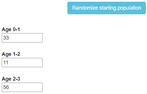
In a population of rabbits,

1. half of the newborn rabbits survive their first year;
2. of those, half survive their second year;
3. the maximum life span is three years;
4. rabbits produce $0$, $6$, $8$ rabbits in their first, second, and third years, respectively.

Let $v_t$ be the vector whose entries $x_t,y_t,z_t$ are the number of rabbits aged $0, 1\text{,}$ and $2\text{,}$ respectively. The rules above can be written as a system of equations:

$$\begin{array}{rrrrrrr}x_{t+1} &=& {}&{}&6y_t &+& 8z_t\\ y_{t+1} &=& \frac 12x_t&{}&{}&{}&{} \\ z_{t+1} &=& {}&{}& \frac 12y_t.&{}&{}\end{array}\nonumber$$

In matrix form, this says:

$$\left(\begin{array}{ccc}0&6&8\\ \frac{1}{2}&0&0\\0&\frac{1}{2}&0\end{array}\right) v_t = v_{t+1}. \nonumber$$

This system is modeled by a difference equation.

Define

$$A = \left(\begin{array}{ccc}0&6&8\\ \frac{1}{2}&0&0\\0&\frac{1}{2}&0\end{array}\right). \nonumber$$

We compute $A$ has eigenvalues $2$ and $-1\text{,}$ and that an eigenvector with eigenvalue $2$ is

$$v = \left(\begin{array}{c}16\\4\\1\end{array}\right). \nonumber$$

This partially explains why the ratio $x_t:y_t:z_t$ approaches $16:4:1$ and why all three quantities eventually double each year in this demo:

Figure $\PageIndex{1}$: Left: the population of rabbits in a given year. Right: the proportions of rabbits in that year. Choose any values you like for the starting population, and click “Advance 1 year” several times. Notice that the ratio $x_t:y_t:z_t$ approaches $16:4:1\text{,}$ and that all three quantities eventually double each year.

Stochastic Matrices and the Steady State

In this subsection, we discuss difference equations representing probabilities, like the Red Box example $\PageIndex{1}$. Such systems are called Markov chains. The most important result in this section is the Perron–Frobenius theorem, which describes the long-term behavior of a Markov chain.

Definition $\PageIndex{2}$: Stochastic

A square matrix $A$ is stochastic if all of its entries are nonnegative, and the entries of each column sum to $1$.

A matrix is positive if all of its entries are positive numbers.

Note $\PageIndex{1}$

A positive stochastic matrix is a stochastic matrix whose entries are all positive numbers. In particular, no entry is equal to zero. For instance, the first matrix below is a positive stochastic matrix, and the second is not:

$$\left(\begin{array}{ccc}.3&.4&.5\\.3&.4&.3\\.4&.2&.2\end{array}\right) \qquad \left(\begin{array}{ccc}1&0&0\\0&1&0\\0&0&1\end{array}\right). \nonumber$$

Remark

More generally, a regular stochastic matrix is a stochastic matrix $A$ such that $A^n$ is positive for some $n \geq 1$. The Perron–Frobenius theorem below also applies to regular stochastic matrices.

Example $\PageIndex{3}$

Continuing with Red Box example $\PageIndex{1}$, the matrix

$$A = \left(\begin{array}{ccc}.3&.4&.5\\.3&.4&.3\\.4&.2&.2\end{array}\right) \nonumber$$

is a positive stochastic matrix. The fact that the columns sum to $1$ says that all of the movies rented from a particular kiosk must be returned to some other kiosk (remember that every customer returns their movie the next day). For instance, the first column says:

Of the movies rented from kiosk $1\text{,}$

$$\begin{split} 30\% \amp\text{ will be returned to kiosk } 1 \\ 30\% \amp\text{ will be returned to kiosk } 2 \\ 40\% \amp\text{ will be returned to kiosk } 3. \\ \end{split} \nonumber$$

The sum is $100\%\text{,}$ as all of the movies are returned to one of the three kiosks.

The matrix $A$ represents the change of state from one day to the next:

$$\left(\begin{array}{c}x_{t+1}\\y_{t+1}\\z_{t+1}\end{array}\right) = A\left(\begin{array}{c}x_t\\y_t\\z_t\end{array}\right) =\left(\begin{array}{c}.3x_t+.4y_t+.5z_t \\ .3x_t+.4y_t+.3z_t \\ .4x_t+.2y_t+.2z_t\end{array}\right). \nonumber$$

If we sum the entries of $v_{t+1}\text{,}$ we obtain

$$\begin{split} \amp(.3x_t+.4y_t+.5z_t)+ (.3x_t+.4y_t+.3z_t)+ (.4x_t+.2y_t+.2z_t) \\ \amp\qquad=(.3+.3+.4)x_t + (.4+.4+.2)y_t + (.5+.3+.2)z_t \\ \amp\qquad= x_t + y_t + z_t. \end{split} \nonumber$$

This says that the total number of copies of Prognosis Negative in the three kiosks does not change from day to day, as we expect.

The fact that the entries of the vectors $v_t$ and $v_{t+1}$ sum to the same number is a consequence of the fact that the columns of a stochastic matrix sum to $1$.

Note $\PageIndex{2}$

Let $A$ be a stochastic matrix, let $v_t$ be a vector, and let $v_{t+1} = Av_t$. Then the sum of the entries of $v_t$ equals the sum of the entries of $v_{t+1}$.

Computing the long-term behavior of a difference equation turns out to be an eigenvalue problem. The eigenvalues of stochastic matrices have very special properties.

Fact $\PageIndex{1}$

Let $A$ be a stochastic matrix. Then:

1. $1$ is an eigenvalue of $A.$
2. If $\lambda$ is a (real or complex) eigenvalue of $A\text{,}$ then $|\lambda|\leq 1.$

Proof

If $A$ is stochastic, then the rows of $A^T$ sum to $1$. But multiplying a matrix by the vector $(1,1,\ldots,1)$ sums the rows:

$$\left(\begin{array}{ccc}.3&.3&.4\\.4&.4&.2\\.5&.3&.2\end{array}\right)\left(\begin{array}{c}1\\1\\1\end{array}\right)=\left(\begin{array}{c}.3+.3+.4\\.4+.4+.2\\.5+.3+.2\end{array}\right)=\left(\begin{array}{c}1\\1\\1\end{array}\right).\nonumber$$

Therefore, $1$ is an eigenvalue of $A^T$. But $A$ and $A^T$ have the same characteristic polynomial:

$$\det(A-\lambda I_n) = \det\bigl((A-\lambda I_n)^T\bigr) = \det(A^T - \lambda I_n). \nonumber$$

Therefore, $1$ is an eigenvalue of $A$.

Now let $\lambda$ be any eigenvalue of $A\text{,}$ so it is also an eigenvalue of $A^T$. Let $x = (x_1,x_2,\ldots,x_n)$ be an eigenvector of $A^T$ with eigenvalue $\lambda\text{,}$ so $\lambda x = A^Tx$. The $j$th entry of this vector equation is

$$\lambda x_j = \sum_{i=1}^n a_{ij} x_i. \nonumber$$

Choose $x_j$ with the largest absolute value, so $|x_i|\leq|x_j|$ for all $i$. Then

$$|\lambda|\cdot|x_j| = \left\vert \sum_{i=1}^n a_{ij} x_i \right\vert \leq \sum_{i=1}^n a_{ij}\cdot |x_i| \leq \sum_{i=1}^n a_{ij}\cdot |x_j| = 1\cdot|x_j|, \nonumber$$

where the last equality holds because $\sum_{i=1}^n a_{ij}=1$. This implies $|\lambda|\leq 1.$

In fact, for a positive stochastic matrix $A\text{,}$ one can show that if $\lambda\neq 1$ is a (real or complex) eigenvalue of $A\text{,}$ then $|\lambda|\lt 1.$ The $1$-eigenspace of a stochastic matrix is very important.

Definition $\PageIndex{3}$: Steady State

A steady state of a stochastic matrix $A$ is an eigenvector $w$ with eigenvalue $1\text{,}$ such that the entries are positive and sum to $1$.

The Perron–Frobenius theorem describes the long-term behavior of a difference equation represented by a stochastic matrix. Its proof is beyond the scope of this text.

Theorem $\PageIndex{1}$: Perron-Frobenius Theorem

Let $A$ be a positive stochastic matrix. Then $A$ admits a unique steady state vector $w\text{,}$ which spans the $1$-eigenspace.

Moreover, for any vector $v_0$ with entries summing to some number $c\text{,}$ the iterates

$$v_1 = Av_0,\; v_2 = Av_1,\; \ldots,\; v_t = Av_{t-1},\; \ldots \nonumber$$

approach $cw$ as $t$ gets large.

Translation: The Perron–Frobenius theorem makes the following assertions:

• The $1$-eigenspace of a positive stochastic matrix is a line.
• The $1$-eigenspace contains a vector with positive entries.
• All vectors approach the $1$-eigenspace upon repeated multiplication by $A$.

One should think of a steady state vector $w$ as a vector of percentages. For example, if the movies are distributed according to these percentages today, then they will be have the same distribution tomorrow, since $Aw=w$. And no matter the starting distribution of movies, the long-term distribution will always be the steady state vector.

The sum $c$ of the entries of $v_0$ is the total number of things in the system being modeled. The total number does not change, so the long-term state of the system must approach $cw\text{:}$ it is a multiple of $w$ because it is contained in the $1$-eigenspace, and the entries of $cw$ sum to $c$.

Recipe 1: Compute the Steady State Vector

Let $A$ be a positive stochastic matrix. Here is how to compute the steady-state vector of $A.$

1. Find any eigenvector $v$ of $A$ with eigenvalue $1$ by solving $(A-I_n)v = 0$.
2. Divide $v$ by the sum of the entries of $v$ to obtain a vector $w$ whose entries sum to $1.$
3. This vector automatically has positive entries. It is the unique steady-state vector.

The above recipe is suitable for calculations by hand, but it does not take advantage of the fact that $A$ is a stochastic matrix. In practice, it is generally faster to compute a steady state vector by computer as follows:

Recipe 2: Approximate the Steady State Vector by Computer

Let $A$ be a positive stochastic matrix. Here is how to approximate the steady-state vector of $A$ with a computer.

1. Choose any vector $v_0$ whose entries sum to $1$ (e.g., a standard coordinate vector).
2. Compute $v_1 = Av_0,\,v_2 = Av_1,\,v_3=Av_2,\,$ etc.
3. These converge to the steady state vector $w$.

Example $\PageIndex{4}$: A $2\times 2$ stochastic matrix

Consider the positive stochastic matrix

$$A = \left(\begin{array}{cc}3/4&1/4 \\ 1/4&3/4\end{array}\right). \nonumber$$

This matrix has characteristic polynomial

$$f(\lambda) = \lambda^2 - \text{Tr}(A)\lambda + \det(\lambda) = \lambda^2 - \frac32\lambda + \frac12  = (\lambda - 1)(\lambda-1/2). \nonumber$$

Notice that $1$ is strictly greater than the other eigenvalue, and that it has algebraic (hence, geometric) multiplicity $1$. We compute eigenvectors for the eigenvalues $1,1/2$ to be, respectively,

$$u_1 = \left(\begin{array}{c}1\\1\end{array}\right) \qquad u_2 = \left(\begin{array}{c}1\\-1\end{array}\right). \nonumber$$

The eigenvector $u_1$ necessarily has positive entries; the steady-state vector is

$$w = \frac 1{1+1}\left(\begin{array}{c}1\\1\end{array}\right) = \frac 12\left(\begin{array}{c}1\\1\end{array}\right) = \left(\begin{array}{c}50\% \\ 50\%\end{array}\right). \nonumber$$

The Perron–Frobenius theorem asserts that, for any vector $v_0\text{,}$ the vectors $v_1 = Av_0,\,v_2=Av_1,\,\ldots$ approach a vector whose entries are the same: $50\%$ of the sum will be in the first entry, and $50\%$ will be in the second.

We can see this explicitly, as follows. The eigenvectors $u_1,u_2$ form a basis $\mathcal{B}$ for $\mathbb{R}^2 \text{;}$ for any vector $x = a_1u_1 + a_2u_2$ in $\mathbb{R}^2 \text{,}$ we have

$$Ax = A(a_1u_1+a_2u_2) = a_1Au_1 + a_2Au_2 = a_1u_1 + \frac{a_2}2u_2. \nonumber$$

Iterating multiplication by $A$ in this way, we have

$$A^tx = a_1u_1 + \frac{a_2}{2^t}u_2 \;\to \; a_1u_1 \nonumber$$

as $t\to\infty$. This shows that $A^tx$ approaches

$$a_1u_1 = \left(\begin{array}{c}a_1 \\ a_1\end{array}\right). \nonumber$$

Note that the sum of the entries of $a_1u_1$ is equal to the sum of the entries of $a_1u_1+a_2u_2\text{,}$ since the entries of $u_2$ sum to $0$.

To illustrate the theorem with numbers, let us choose a particular value for $u_0\text{,}$ say $u_0={1\choose 0}$. We compute the values for $u_t = {x_t\choose y_t}$ in this table:

$$\begin{array}{c|c|c|c} t & x_t & y_t \\\hline 0 & 1.000 & 0.000 \\ 1 & 0.750 & 0.250 \\ 2 & 0.625 & 0.375 \\ 3 & 0.563 & 0.438 \\ 4 & 0.531 & 0.469 \\ 5 & 0.516 & 0.484 \\ 6 & 0.508 & 0.492 \\ 7 & 0.504 & 0.496 \\ 8 & 0.502 & 0.498 \\ 9 & 0.501 & 0.499 \\ 10& 0.500 & 0.500 \\ \end{array} \nonumber$$

We see that $u_t$ does indeed approach ${0.5\choose0.5}$.

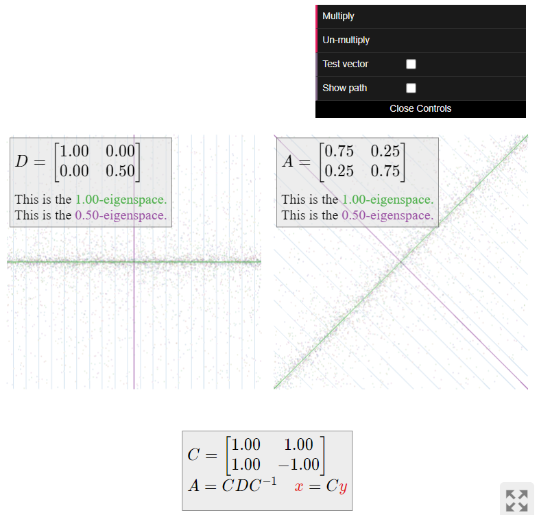
Now we turn to visualizing the dynamics of (i.e., repeated multiplication by) the matrix $A$. This matrix is diagonalizable; we have $A=CDC^{-1}$ for

$$C = \left(\begin{array}{cc}1&1\\1&-1\end{array}\right) \qquad D = \left(\begin{array}{cc}1&0\\0&1/2\end{array}\right). \nonumber$$

The matrix $D$ leaves the $x$-coordinate unchanged and scales the $y$-coordinate by $1/2$. Repeated multiplication by $D$ makes the $y$-coordinate very small, so it “sucks all vectors into the $x$-axis.”

The matrix $A$ does the same thing as $D\text{,}$ but with respect to the coordinate system defined by the columns $u_1,u_2$ of $C$. This means that $A$ “sucks all vectors into the $1$-eigenspace”, without changing the sum of the entries of the vectors.

Figure $\PageIndex{2}$: Dynamics of the stochastic matrix $A$. Click “multiply” to multiply the colored points by $D$ on the left and $A$ on the right. Note that on both sides, all vectors are “sucked into the $1$-eigenspace” (the red line).

Example $\PageIndex{5}$

Continuing with Red Box example $\PageIndex{1}$, we can illustrate the Perron–Frobenius theorem explicitly. The matrix

$$A = \left(\begin{array}{ccc}.3&.4&.5\\.3&.4&.3\\.4&.2&.2\end{array}\right) \nonumber$$

has characteristic polynomial

$$f(\lambda) = -\lambda^3 + 0.12\lambda - 0.02 = -(\lambda-1)(\lambda+0.2)(\lambda-0.1). \nonumber$$

Notice that $1$ is strictly greater in absolute value than the other eigenvalues, and that it has algebraic (hence, geometric) multiplicity $1$. We compute eigenvectors for the eigenvalues $1,-0.2,0.1$ to be, respectively,

$$u_1 = \left(\begin{array}{c}7\\6\\5\end{array}\right) \qquad u_2 = \left(\begin{array}{c}-1\\0\\1\end{array}\right) \qquad u_3 = \left(\begin{array}{c}1\\-3\\2\end{array}\right). \nonumber$$

The eigenvector $u_1$ necessarily has positive entries; the steady-state vector is

$$w = \frac 1{7+6+5}u_1 = \frac 1{18}\left(\begin{array}{c}7\\6\\5\end{array}\right). \nonumber$$

The eigenvectors $u_1,u_2,u_3$ form a basis $\mathcal{B}$ for $\mathbb{R}^3 \text{;}$ for any vector $x = a_1u_1+a_2u_2+a_3u_3$ in $\mathbb{R}^3 \text{,}$ we have

$$\begin{split} Ax \amp= A(a_1u_1+a_2u_2+a_3u_3) \\ \amp= a_1Au_1 + a_2Au_2 + a_3Au_3 \\ \amp= a_1u_1 - 0.2a_2u_2 + 0.1a_3u_3. \end{split} \nonumber$$

Iterating multiplication by $A$ in this way, we have

$$A^tx = a_1u_1 - (0.2)^ta_2u_2 + (0.1)^ta_3u_3 \;\to \; a_1u_1 \nonumber$$

as $t\to\infty$. This shows that $A^tx$ approaches $a_1u_1\text{,}$ which is an eigenvector with eigenvalue $1$, as guaranteed by the Perron–Frobenius theorem.

What do the above calculations say about the number of copies of Prognosis Negative in the Atlanta Red Box kiosks? Suppose that the kiosks start with 100 copies of the movie, with $30$ copies at kiosk 1, $50$ copies at kiosk $2\text{,}$ and $20$ copies at kiosk $3$. Let $v_0 = (30,50,20)$ be the vector describing this state. Then there will be $v_1 = Av_0$ movies in the kiosks the next day, $v_2 = Av_1$ the day after that, and so on. We let $v_t = (x_t,y_t,z_t).$

$$\begin{array}{c|c|c|c} t & x_t & y_t & z_t \\\hline 0 & 30.000000 & 50.000000 & 20.000000 \\ 1 & 39.000000 & 35.000000 & 26.000000 \\ 2 & 38.700000 & 33.500000 & 27.800000 \\ 3 & 38.910000 & 33.350000 & 27.740000 \\ 4 & 38.883000 & 33.335000 & 27.782000 \\ 5 & 38.889900 & 33.333500 & 27.776600 \\ 6 & 38.888670 & 33.333350 & 27.777980 \\ 7 & 38.888931 & 33.333335 & 27.777734 \\ 8 & 38.888880 & 33.333333 & 27.777786 \\ 9 & 38.888891 & 33.333333 & 27.777776 \\ 10& 38.888889 & 33.333333 & 27.777778 \\ \end{array} \nonumber$$

(Of course it does not make sense to have a fractional number of movies; the decimals are included here to illustrate the convergence.) The steady-state vector says that eventually, the movies will be distributed in the kiosks according to the percentages

$$w = \frac 1{18}\left(\begin{array}{c}7\\6\\5\end{array}\right) = \left(\begin{array}{c}38.888888\% \\ 33.333333\% \\ 27.777778\%\end{array}\right), \nonumber$$

which agrees with the above table. Moreover, this distribution is independent of the beginning distribution of movies in the kiosks.

Now we turn to visualizing the dynamics of (i.e., repeated multiplication by) the matrix $A$. This matrix is diagonalizable; we have $A=CDC^{-1}$ for

$$C = \left(\begin{array}{ccc}7&-1&1\\6&0&-3\\5&1&2\end{array}\right) \qquad D = \left(\begin{array}{ccc}1&0&0\\0&-.2&0\\0&0&.1\end{array}\right). \nonumber$$

The matrix $D$ leaves the $x$-coordinate unchanged, scales the $y$-coordinate by $-1/5\text{,}$ and scales the $z$-coordinate by $1/10$. Repeated multiplication by $D$ makes the $y$- and $z$-coordinates very small, so it “sucks all vectors into the $x$-axis.”

The matrix $A$ does the same thing as $D\text{,}$ but with respect to the coordinate system defined by the columns $u_1,u_2,u_3$ of $C$. This means that $A$ “sucks all vectors into the $1$-eigenspace”, without changing the sum of the entries of the vectors.

Figure $\PageIndex{3}$: Dynamics of the stochastic matrix $A$. Click “multiply” to multiply the colored points by $D$ on the left and $A$ on the right. Note that on both sides, all vectors are “sucked into the $1$-eigenspace” (the green line). (We have scaled $C$ by $1/4$ so that vectors have roughly the same size on the right and the left. The “jump” that happens when you press “multiply” is a negation of the $-.2$-eigenspace, which is not animated.)

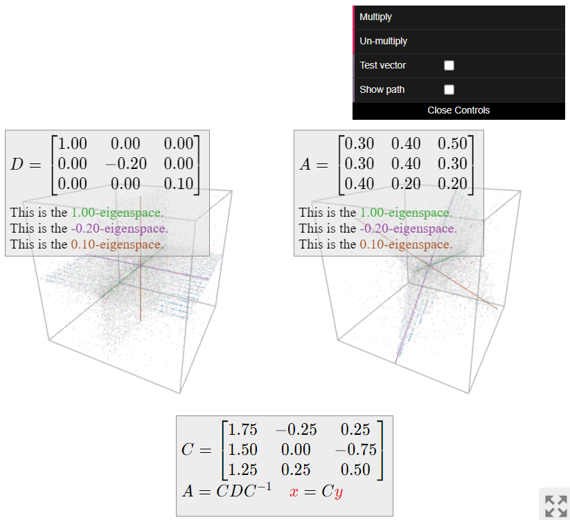
The picture of a positive stochastic matrix is always the same, whether or not it is diagonalizable: all vectors are “sucked into the $1$-eigenspace,” which is a line, without changing the sum of the entries of the vectors. This is the geometric content of the Perron–Frobenius theorem.

Google’s PageRank Algorithm

Internet searching in the 1990s was very inefficient. Yahoo or AltaVista would scan pages for your search text, and simply list the results with the most occurrences of those words. Not surprisingly, the more unsavory websites soon learned that by putting the words “Alanis Morissette” a million times in their pages, they could show up first every time an angsty teenager tried to find Jagged Little Pill on Napster.

Larry Page and Sergey Brin invented a way to rank pages by importance. They founded Google based on their algorithm. Here is roughly how it works.

Each web page has an associated importance, or rank. This is a positive number. This rank is determined by the following rule.

Definition $\PageIndex{4}$: The Importance Rule

If a page $P$ links to $n$ other pages $Q_1,Q_2,\ldots,Q_n\text{,}$ then each page $Q_i$ inherits $\frac 1n$ of $P$’s importance.

In practice, this means:

• If a very important page links to your page (and not to a zillion other ones as well), then your page is considered important.
• If a zillion unimportant pages link to your page, then your page is still important.
• If only one unknown page links to yours, your page is not important.

Alternatively, there is the random surfer interpretation. A “random surfer” just sits at his computer all day, randomly clicking on links. The pages he spends the most time on should be the most important. So, the important (high-ranked) pages are those where a random surfer will end up most often. This measure turns out to be equivalent to the rank.

Definition $\PageIndex{5}$: The Importance Matrix

Consider an internet with $n$ pages. The importance matrix is the $n\times n$ matrix $A$ whose $i,j$-entry is the importance that page $j$ passes to page $i.$

Observe that the importance matrix is a stochastic matrix, assuming every page contains a link: if page $i$ has $m$ links, then the $i$th column contains the number $1/m\text{,}$ $m$ times, and the number zero in the other entries.

Example $\PageIndex{6}$

Consider the following internet with only four pages. Links are indicated by arrows.

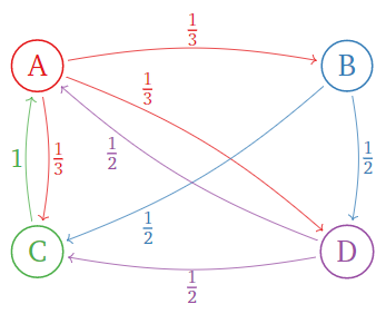
Figure $\PageIndex{4}$

The importance rule says:

• Page $\color{Red}A$ has $3$ links, so it passes $\frac 13$ of its importance to pages $B,C,D$.
• Page $\color{blue}B$ has $2$ links, so it passes $\frac 12$ of its importance to pages $C,D$.
• Page $\color{Green}C$ has one link, so it passes all of its importance to page $A$.
• Page $\color{Purple}D$ has $2$ links, so it passes $\frac 12$ of its importance to pages $A,C$.

In terms of matrices, if $v = (a,b,c,d)$ is the vector containing the ranks $a,b,c,d$ of the pages $A,B,C,D\text{,}$ then

$$\left(\begin{array}{cccc}\color{Red}{0}&\color{blue}{0}&\color{Green}{1}&\color{Purple}{\frac{1}{2}} \\ \color{Red}{\frac{1}{3}}&\color{blue}{0}&\color{Green}{0}&\color{Purple}{0} \\ \color{Red}{\frac{1}{3}}&\color{blue}{\frac{1}{2}}&\color{Green}{0}&\color{Purple}{\frac{1}{2}} \\ \color{Red}{\frac{1}{3}}&\color{blue}{\frac{1}{2}}&\color{Green}{0}&\color{Purple}{0}\end{array}\right)\left(\begin{array}{c}a\\b\\c\\d\end{array}\right)=\left(\begin{array}{lr}{}&{c+\frac{1}{2}d} \\ {\frac{1}{3}a}&{}\\ {\frac{1}{3}a+\frac{1}{2}b}&{+\frac{1}{2}d} \\ {\frac{1}{3}a+\frac{1}{2}b}&{}\end{array}\right)=\left(\begin{array}{c}a\\b\\c\\d\end{array}\right).\nonumber$$

The matrix on the left is the importance matrix, and the final equality expresses the importance rule.

The above example illustrates the key observation.

Key Observation $\PageIndex{1}$

The rank vector is an eigenvector of the importance matrix with eigenvalue $1$.

In light of the key observation, we would like to use the Perron–Frobenius theorem to find the rank vector. Unfortunately, the importance matrix is not always a positive stochastic matrix.

Example $\PageIndex{7}$: A page with no links

Consider the following internet with three pages:

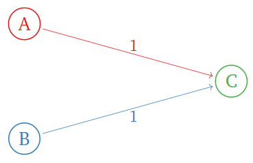
Figure $\PageIndex{5}$

The importance matrix is

$$\left(\begin{array}{ccc}\color{Red}{0}&\color{blue}{0}&\color{Green}{0} \\ \color{Red}{0}&\color{blue}{0}&\color{Green}{0} \\ \color{Red}{1}&\color{blue}{1}&\color{Green}{0}\end{array}\right).\nonumber$$

This has characteristic polynomial

$$f(\lambda) = \det\left(\begin{array}{ccc}-\lambda&0&0\\ 0&-\lambda&0 \\ 1&1&-\lambda\end{array}\right) = -\lambda^3. \nonumber$$

So $1$ is not an eigenvalue at all: there is no rank vector! The importance matrix is not stochastic because the page $C$ has no links.

Example $\PageIndex{8}$: Disconnected Internet

Consider the following internet:

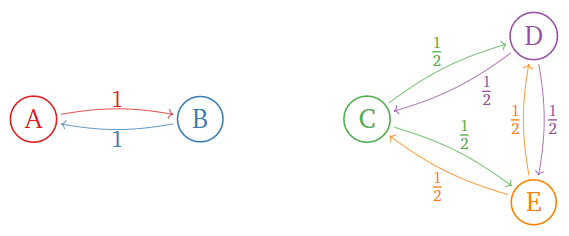
Figure $\PageIndex{6}$

The importance matrix is

$$\left(\begin{array}{ccccc}\color{Red}{0}&\color{blue}{1}&\color{black}{0}&0&0\\ \color{Red}{1}&\color{blue}{0}&\color{black}{0}&0&0 \\ 0&0&\color{Green}{0}&\color{Purple}{\frac{1}{2}}&\color{orange}{\frac{1}{2}} \\ 0&0&\color{Green}{\frac{1}{2}}&\color{Purple}{0}&\color{orange}{\frac{1}{2}} \\ 0&0&\color{Green}{\frac{1}{2}}&\color{Purple}{\frac{1}{2}}&\color{orange}{0}\end{array}\right).\nonumber$$

This has linearly independent eigenvectors

$$\left(\begin{array}{c}1\\1\\0\\0\\0\end{array}\right)\quad\text{and}\quad\left(\begin{array}{c}0\\0\\1\\1\\1\end{array}\right),\nonumber$$

both with eigenvalue $1$. So there is more than one rank vector in this case. Here the importance matrix is stochastic, but not positive.

Here is Page and Brin’s solution. First we fix the importance matrix by replacing each zero column with a column of $1/n$s, where $n$ is the number of pages:

$$A=\left(\begin{array}{ccc}0&0&0\\0&0&0\\1&1&0\end{array}\right)\quad\text{becomes}\quad A'=\left(\begin{array}{ccc}0&0&1/3 \\ 0&0&1/3 \\ 1&1&1/3\end{array}\right).\nonumber$$

The modified importance matrix $A'$ is always stochastic.

Now we choose a number $p$ in $(0,1)\text{,}$ called the damping factor. (A typical value is $p=0.15$.)

Definition $\PageIndex{6}$: The Google Matrix

Let $A$ be the importance matrix for an internet with $n$ pages, and let $A'$ be the modified importance matrix. The Google Matrix is the matrix

$$M = (1-p)\cdot A' + p\cdot B \quad\text{where}\quad B = \frac 1n\left(\begin{array}{cccc}1&1&\cdot &1 \\ 1&1&\cdot &1 \\ \vdots&\vdots&\ddots&\vdots \\ 1&1&\cdots &1\end{array}\right). \nonumber$$

In the random surfer interpretation, this matrix $M$ says: with probability $p\text{,}$ our surfer will surf to a completely random page; otherwise, he'll click a random link on the current page, unless the current page has no links, in which case he'll surf to a completely random page in either case. The reader can verify the following important fact.

Fact $\PageIndex{2}$

The Google Matrix is a positive stochastic matrix.

If we declare that the ranks of all of the pages must sum to $1\text{,}$ then we find:

Note $\PageIndex{3}$: The 25 Billion Dollar Eigenvector

The PageRank vector is the steady state of the Google Matrix.

This exists and has positive entries by the Perron–Frobenius theorem. The hard part is calculating it: in real life, the Google Matrix has zillions of rows.

Example $\PageIndex{9}$: PageRank Vector

What is the PageRank vector for the following internet? (Use the damping factor $p = 0.15$.)

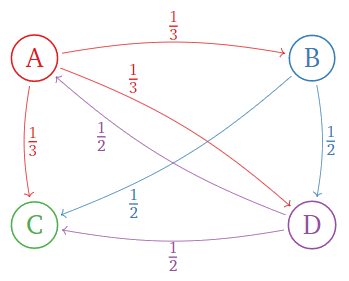
Figure $\PageIndex{7}$

Which page is the most important? Which is the least important?

Solution

First we compute the modified importance matrix:

$$A=\left(\begin{array}{cccc}\color{Red}{0}&\color{blue}{0}&\color{Green}{0}&\color{Purple}{\frac{1}{2}} \\ \color{Red}{\frac{1}{3}}&\color{blue}{0}&\color{Green}{0}&\color{Purple}{0} \\ \color{Red}{\frac{1}{3}}&\color{blue}{\frac{1}{2}}&\color{Green}{0}&\color{Purple}{\frac{1}{2}} \\ \color{Red}{\frac{1}{3}}&\color{blue}{\frac{1}{2}}&\color{Green}{0}&\color{Purple}{0}\end{array}\right) \quad\xrightarrow{\text{modify}}\quad A'=\left(\begin{array}{cccc}\color{Red}{0}&\color{blue}{0}&\color{Green}{\frac{1}{4}}&\color{Purple}{\frac{1}{2}} \\ \color{Red}{\frac{1}{3}}&\color{blue}{0}&\color{Green}{\frac{1}{4}}&\color{Purple}{0} \\ \color{Red}{\frac{1}{3}}&\color{blue}{\frac{1}{2}}&\color{Green}{\frac{1}{4}}&\color{Purple}{\frac{1}{2}} \\ \color{Red}{\frac{1}{3}}&\color{blue}{\frac{1}{2}}&\color{Green}{\frac{1}{4}}&\color{Purple}{0}\end{array}\right)\nonumber$$

Choosing the damping factor $p=0.15\text{,}$ the Google Matrix is

$$\begin{align*} M &=0.85\cdot\left(\begin{array}{cccc}\color{Red}{0}&\color{blue}{0}&\color{Green}{\frac{1}{4}}&\color{Purple}{\frac{1}{2}} \\ \color{Red}{\frac{1}{3}}&\color{blue}{0}&\color{Green}{\frac{1}{4}}&\color{Purple}{0} \\ \color{Red}{\frac{1}{3}}&\color{blue}{\frac{1}{2}}&\color{Green}{\frac{1}{4}}&\color{Purple}{\frac{1}{2}} \\ \color{Red}{\frac{1}{3}}&\color{blue}{\frac{1}{2}}&\color{Green}{\frac{1}{4}}&\color{Purple}{0}\end{array}\right)+0.15\cdot\left(\begin{array}{cccc}1/4&1/4&1/4&1/4 \\ 1/4&1/4&1/4&1/4 \\1/4&1/4&1/4&1/4 \\1/4&1/4&1/4&1/4  \end{array}\right) \\[4pt] &\approx\left(\begin{array}{cccc}0.0375& 0.0375& 0.2500 &0.4625\\ 0.3208& 0.0375& 0.2500& 0.0375\\ 0.3208& 0.4625 &0.2500& 0.4625\\ 0.3208 &0.4625& 0.2500& 0.0375\end{array}\right).\end{align*}\nonumber$$

The PageRank vector is the steady state:

$$w \approx \left(\begin{array}{c}0.2192\\ 0.1752 \\0.3558\\ 0.2498\end{array}\right) \nonumber$$

This is the PageRank:

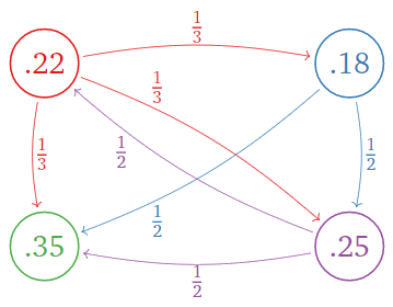
Figure $\PageIndex{8}$

Page $C$ is the most important, with a rank of $0.558\text{,}$ and page $B$ is the least important, with a rank of $0.1752.$