5.5: Complex Eigenvalues

$\usepackage{macros} \newcommand{\lt}{<} \newcommand{\gt}{>} \newcommand{\amp}{&}$

Objectives

1. Learn to find complex eigenvalues and eigenvectors of a matrix.
2. Learn to recognize a rotation-scaling matrix, and compute by how much the matrix rotates and scales.
3. Understand the geometry of $2\times 2$ and $3\times 3$ matrices with a complex eigenvalue.
4. Recipes: a $2\times 2$ matrix with a complex eigenvalue is similar to a rotation-scaling matrix, the eigenvector trick for $2\times 2$ matrices.
5. Pictures: the geometry of matrices with a complex eigenvalue.
6. Theorems: the rotation-scaling theorem, the block diagonalization theorem.
7. Vocabulary word: rotation-scaling matrix.

In Section 5.4, we saw that an $n \times n$ matrix whose characteristic polynomial has $n$ distinct real roots is diagonalizable: it is similar to a diagonal matrix, which is much simpler to analyze. The other possibility is that a matrix has complex roots, and that is the focus of this section. It turns out that such a matrix is similar (in the $2\times 2$ case) to a rotation-scaling matrix, which is also relatively easy to understand.

In a certain sense, this entire section is analogous to Section 5.4, with rotation-scaling matrices playing the role of diagonal matrices. See Section 7.1 for a review of the complex numbers.

Matrices with Complex Eigenvalues

As a consequence of the fundamental theorem of algebra, Theorem 7.1.1 in Section 7.1, as applied to the characteristic polynomial, we see that:

Note $\PageIndex{1}$

Every $n \times n$ matrix has exactly $n$ complex eigenvalues, counted with multiplicity.

We can compute a corresponding (complex) eigenvector in exactly the same way as before: by row reducing the matrix $A - \lambda I_n$. Now, however, we have to do arithmetic with complex numbers.

Example $\PageIndex{1}$: A $2\times 2$ matrix

Find the complex eigenvalues and eigenvectors of the matrix

$$A = \left(\begin{array}{cc}1&-1\\1&1\end{array}\right). \nonumber$$

Solution

The characteristic polynomial of $A$ is

$$f(\lambda) = \lambda^2 - \text{Tr}(A)\lambda + \det(A) = \lambda^2 - 2\lambda + 2. \nonumber$$

The roots of this polynomial are

$$\lambda = \frac{2\pm\sqrt{4-8}}2 = 1\pm i. \nonumber$$

First we compute an eigenvector for $\lambda = 1+i$. We have

$$A-(1+i) I_2 = \left(\begin{array}{cc}1-(1+i)&-1 \\ 1&1-(1+i) \end{array}\right) = \left(\begin{array}{cc}-i&-1\\1&-i\end{array}\right). \nonumber$$

Now we row reduce, noting that the second row is $i$ times the first:

$$\left(\begin{array}{cc}-i&-1\\1&-i\end{array}\right) \;\xrightarrow{R_2=R_2-iR_1}\; \left(\begin{array}{cc}-i&-1\\0&0\end{array}\right) \;\xrightarrow{R_1=R_1\div -i}\; \left(\begin{array}{cc}1&-i\\0&0\end{array}\right). \nonumber$$

The parametric form is $x = iy\text{,}$ so that an eigenvector is $v_1={i\choose 1}$. Next we compute an eigenvector for $\lambda=1-i$. We have

$$A-(1-i) I_2 = \left(\begin{array}{cc}1-(1-i)&-1\\1&1-(1-i)\end{array}\right) = \left(\begin{array}{cc}i&-1\\1&i\end{array}\right). \nonumber$$

Now we row reduce, noting that the second row is $-i$ times the first:

$$\left(\begin{array}{cc}i&-1\\1&i\end{array}\right) \;\xrightarrow{R_2=R_2+iR_1}\; \left(\begin{array}{cc}i&-1\\0&0\end{array}\right) \;\xrightarrow{R_1=R_1\div i}\; \left(\begin{array}{cc}1&i\\0&0\end{array}\right). \nonumber$$

The parametric form is $x = -iy\text{,}$ so that an eigenvector is $v_2 = {-i\choose 1}$.

We can verify our answers:

$$\begin{aligned}\left(\begin{array}{cc}1&-1\\1&1\end{array}\right)\left(\begin{array}{c}i\\1\end{array}\right)&=\left(\begin{array}{c}i-1\\i+1\end{array}\right)=(1+i)\left(\begin{array}{c}i\\1\end{array}\right) \\ \left(\begin{array}{cc}1&-1\\1&1\end{array}\right)\left(\begin{array}{c}-i\\1\end{array}\right)&=\left(\begin{array}{c}-i-1\\-i+1\end{array}\right)=(1-i)\left(\begin{array}{c}-i\\1\end{array}\right).\end{aligned}$$

Example $\PageIndex{2}$: A $3\times 3$ matrix

Find the eigenvalues and eigenvectors, real and complex, of the matrix

$$A=\left(\begin{array}{ccc}4/5&-3/5&0 \\ 3/5&4/5&0\\1&2&2\end{array}\right).\nonumber$$

Solution

We compute the characteristic polynomial by expanding cofactors along the third row:

$$f(\lambda) = \det\left(\begin{array}{ccc}4/5-\lambda &-3/5&0 \\ 3/5&4-5-\lambda &0 \\ 1&2&2-\lambda\end{array}\right) = (2-\lambda)\left(\lambda^2-\frac 85\lambda+1\right). \nonumber$$

This polynomial has one real root at $2\text{,}$ and two complex roots at

$$\lambda = \frac{8/5\pm\sqrt{64/25-4}}2 = \frac{4\pm 3i}5. \nonumber$$

Therefore, the eigenvalues are

$$\lambda = 2,\quad \frac{4+3i}5,\quad \frac{4-3i}5. \nonumber$$

We eyeball that $v_1 = e_3$ is an eigenvector with eigenvalue $2\text{,}$ since the third column is $2e_3$.

Next we find an eigenvector with eigenvaluue $(4+3i)/5$. We have

$$A-\frac{4+3i}5I_3 = \left(\begin{array}{ccc}-3i/5&-3/5&0\\3/5&-3i/5&0\\ 1&2&2-(4+3i)/5\end{array}\right) \;\xrightarrow[R_2=R_2\times5/3]{R_1=R_1\times -5/3}\; \left(\begin{array}{ccc}i&1&0\\1&-i&0\\1&2&\frac{6-3i}{5}\end{array}\right). \nonumber$$

We row reduce, noting that the second row is $-i$ times the first:

$$\begin{aligned}\left(\begin{array}{ccc}i&1&0\\1&-i&0\\1&2&\frac{6-3i}{5}\end{array}\right)\xrightarrow{R_2=R_2+iR_1}\quad &\left(\begin{array}{ccc}i&1&0\\0&0&0\\1&2&\frac{6-3i}{5}\end{array}\right) \\ {}\xrightarrow{R_3=R_3+iR_1}\quad &\left(\begin{array}{ccc}i&1&0\\0&0&0\\0&2+i&\frac{6-3i}{5}\end{array}\right) \\ {}\xrightarrow{R_2\longleftrightarrow R_3}\quad &\left(\begin{array}{ccc}i&1&0\\0&2+i&\frac{6-3i}{5}\\0&0&0\end{array}\right) \\ {}\xrightarrow[R_2=R_2\div(2+i)]{R_1=R_1\div i}\quad &\left(\begin{array}{ccc}1&-i&0\\0&1&\frac{9-12i}{25}\\0&0&0\end{array}\right) \\ {}\xrightarrow{R_1=R_1+iR_2}\quad &\left(\begin{array}{ccc}1&0&\frac{12+9i}{25}\\0&1&\frac{9-12i}{25}\\0&0&0\end{array}\right).\end{aligned}$$

The free variable is $z\text{;}$ the parametric form of the solution is

$$\left\{\begin{array}{rrr}x &=& -\dfrac{12+9i}{25}z \\ y &=& -\dfrac{9-12i}{25}z.\end{array}\right.\nonumber$$

Taking $z=25$ gives the eigenvector

$$v_2 = \left(\begin{array}{c}-12-9i\\-9+12i\\25\end{array}\right). \nonumber$$

A similar calculation (replacing all occurences of $i$ by $-i$) shows that an eigenvector with eigenvalue $(4-3i)/5$ is

$$v_3 = \left(\begin{array}{c}-12+9i\\-9-12i\\25\end{array}\right). \nonumber$$

We can verify our calculations:

$$\begin{aligned}\left(\begin{array}{ccc}4/5&-3/5&0\\3/5&4/5&0\\1&2&2\end{array}\right)\left(\begin{array}{c}-12+9i\\-9-12i\\25\end{array}\right)&=\left(\begin{array}{c}-21/5+72i/5 \\ -72/5-21i/5\\20-15i\end{array}\right)=\frac{4+3i}{5}\left(\begin{array}{c}-12+9i\\-9-12i\\25\end{array}\right) \\ \left(\begin{array}{ccc}4/5&-3/5&0\\3/5&4/5&0\\1&2&2\end{array}\right)\left(\begin{array}{c}-12-9i\\-9+12i\\25\end{array}\right)&=\left(\begin{array}{c}-21/5-72i/5\\-72/5+21i/5\\20+15i\end{array}\right)=\frac{4-3i}{5}\left(\begin{array}{c}-12-9i\\-9+12i\\25\end{array}\right).\end{aligned}$$

If $A$ is a matrix with real entries, then its characteristic polynomial has real coefficients, so Note 7.1.3 in Section 7.1 implies that its complex eigenvalues come in conjugate pairs. In the first example, we notice that

$$\begin{split} 1+i \text{ has an eigenvector } \amp v_1 =\left(\begin{array}{c}i\\1\end{array}\right) \\ 1-i \text{ has an eigenvector } \amp v_2 = \left(\begin{array}{c}-i\\1\end{array}\right). \end{split} \nonumber$$

In the second example,

$$\begin{split} \frac{4+3i}5 \text{ has an eigenvector } \amp v_1 = \left(\begin{array}{c}-12-9i\\-9+12i\\25\end{array}\right) \\ \frac{4-3i}5 \text{ has an eigenvector } \amp v_2 =\left(\begin{array}{c}-12+9i\\-9-12i\\25\end{array}\right) \end{split} \nonumber$$

In these cases, an eigenvector for the conjugate eigenvalue is simply the conjugate eigenvector (the eigenvector obtained by conjugating each entry of the first eigenvector). This is always true. Indeed, if $Av=\lambda v$ then

$$A \bar v = \bar{Av} = \bar{\lambda v} = \bar \lambda \bar v, \nonumber$$

which exactly says that $\bar v$ is an eigenvector of $A$ with eigenvalue $\bar \lambda$.

Note $\PageIndex{2}$

Let $A$ be a matrix with real entries. If

$$\begin{split} \lambda \text{ is a complex eigenvalue with eigenvector } \amp v, \\ \text{then } \bar\lambda \text{ is a complex eigenvalue with eigenvector }\amp\bar v. \end{split} \nonumber$$

In other words, both eigenvalues and eigenvectors come in conjugate pairs.

Since it can be tedious to divide by complex numbers while row reducing, it is useful to learn the following trick, which works equally well for matrices with real entries.

Note $\PageIndex{3}$: Eigenvector Trick for $2\times 2$ Matrices

Let $A$ be a $2\times 2$ matrix, and let $\lambda$ be a (real or complex) eigenvalue. Then

$$A - \lambda I_2 = \left(\begin{array}{cc}z&w\\ \star&\star\end{array}\right) \quad\implies\quad \left(\begin{array}{c}-w\\z\end{array}\right) \text{ is an eigenvector with eigenvalue } \lambda, \nonumber$$

assuming the first row of $A-\lambda I_2$ is nonzero.

Indeed, since $\lambda$ is an eigenvalue, we know that $A-\lambda I_2$ is not an invertible matrix. It follows that the rows are collinear (otherwise the determinant is nonzero), so that the second row is automatically a (complex) multiple of the first:

$$\left(\begin{array}{cc}z&w\\ \star&\star\end{array}\right)=\left(\begin{array}{cc}z&w\\cz&cw\end{array}\right).\nonumber$$

It is obvious that ${-w\choose z}$ is in the null space of this matrix, as is ${w\choose -z}\text{,}$ for that matter. Note that we never had to compute the second row of $A-\lambda I_2\text{,}$ let alone row reduce!

Example $\PageIndex{3}$: A $2\times 2$ matrix, the easy way

Find the complex eigenvalues and eigenvectors of the matrix

$$A = \left(\begin{array}{cc}1&-1\\1&1\end{array}\right). \nonumber$$

Solution

Since the characteristic polynomial of a $2\times 2$ matrix $A$ is $f(\lambda) = \lambda^2-\text{Tr}(A)\lambda + \det(A)\text{,}$ its roots are

$$\lambda = \frac{\text{Tr}(A)\pm\sqrt{\text{Tr}(A)^2-4\det(A)}}2 = \frac{2\pm\sqrt{4-8}}2 = 1\pm i. \nonumber$$

To find an eigenvector with eigenvalue $1+i\text{,}$ we compute

$$A - (1+i)I_2 = \left(\begin{array}{cc}-i&-1\\ \star&\star\end{array}\right) \;\xrightarrow{\text{eigenvector}}\; v_1 = \left(\begin{array}{c}1\\-i\end{array}\right). \nonumber$$

The eigenvector for the conjugate eigenvalue is the complex conjugate:

$$v_2 = \bar v_1 = \left(\begin{array}{c}1\\i\end{array}\right). \nonumber$$

In Example $\PageIndex{1}$ we found the eigenvectors ${i\choose 1}$ and ${-i\choose 1}$ for the eigenvalues $1+i$ and $1-i\text{,}$ respectively, but in Example $\PageIndex{3}$ we found the eigenvectors ${1\choose -i}$ and ${1\choose i}$ for the same eigenvalues of the same matrix. These vectors do not look like multiples of each other at first—but since we now have complex numbers at our disposal, we can see that they actually are multiples:

$$-i\left(\begin{array}{c}i\\1\end{array}\right) = \left(\begin{array}{c}1\\-i\end{array}\right) \qquad i\left(\begin{array}{c}-i\\1\end{array}\right) = \left(\begin{array}{c}1\\i\end{array}\right). \nonumber$$

Rotation-Scaling Matrices

The most important examples of matrices with complex eigenvalues are rotation-scaling matrices, i.e., scalar multiples of rotation matrices.

Definition $\PageIndex{1}$: Rotation-Scaling matrix

A rotation-scaling matrix is a $2\times 2$ matrix of the form

$$\left(\begin{array}{cc}a&-b\\b&a\end{array}\right), \nonumber$$

where $a$ and $b$ are real numbers, not both equal to zero.

The following proposition justifies the name.

Proposition $\PageIndex{1}$

Let $$A = \left(\begin{array}{cc}a&-b\\b&a\end{array}\right) \nonumber$$ be a rotation-scaling matrix. Then:

1. $A$ is a product of a rotation matrix $$\left(\begin{array}{cc}\cos\theta&-\sin\theta \\ \sin\theta&\cos\theta\end{array}\right)\quad\text{with a scaling matrix}\quad\left(\begin{array}{cc}r&0\\0&r\end{array}\right).\nonumber$$
2. The scaling factor $r$ is  $$r = \sqrt{\det(A)} = \sqrt{a^2+b^2}. \nonumber$$
3. The rotation angle $\theta$ is the counterclockwise angle from the positive $x$-axis to the vector ${a\choose b}\text{:}$ 

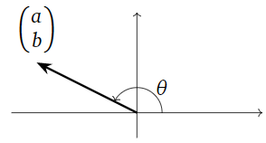
Figure $\PageIndex{1}$

The eigenvalues of $A$ are $\lambda = a \pm bi.$

Proof

Set $r = \sqrt{\det(A)} = \sqrt{a^2+b^2}$. The point $(a/r, b/r)$ has the property that

$$\left(\frac ar\right)^2 + \left(\frac br\right)^2 = \frac{a^2+b^2}{r^2} = 1. \nonumber$$

In other words $(a/r,b/r)$ lies on the unit circle. Therefore, it has the form $(\cos\theta,\sin\theta)\text{,}$ where $\theta$ is the counterclockwise angle from the positive $x$-axis to the vector ${a/r\choose b/r}\text{,}$ or since it is on the same line, to ${a\choose b}\text{:}$

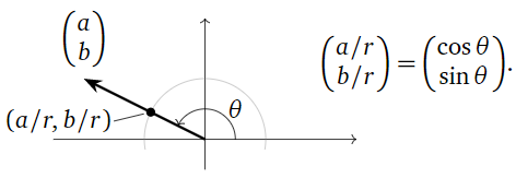
Figure $\PageIndex{2}$

It follows that

$$A = r\left(\begin{array}{cc}a/r&-b/r \\ b/r&a/r\end{array}\right) =\left(\begin{array}{cc}r&0\\0&r\end{array}\right) \left(\begin{array}{cc}\cos\theta&-\sin\theta \\ \sin\theta&\cos\theta\end{array}\right), \nonumber$$

as desired.

For the last statement, we compute the eigenvalues of $A$ as the roots of the characteristic polynomial:

$$\lambda = \frac{\text{Tr}(A)\pm\sqrt{\text{Tr}(A)^2-4\det(A)}}2 = \frac{2a\pm\sqrt{4a^2-4(a^2+b^2)}}2 = a\pm bi. \nonumber$$

Geometrically, a rotation-scaling matrix does exactly what the name says: it rotates and scales (in either order).

Example $\PageIndex{4}$: A rotation-scaling matrix

What does the matrix

$$A = \left(\begin{array}{cc}1&-1\\1&1\end{array}\right) \nonumber$$

do geometrically?

Solution

This is a rotation-scaling matrix with $a=b=1$. Therefore, it scales by a factor of $\sqrt{\det(A)} = \sqrt 2$ and rotates counterclockwise by $45^\circ\text{:}$

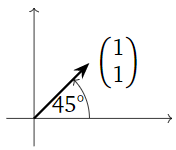
Figure $\PageIndex{3}$

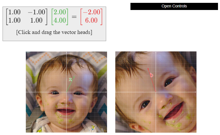
Here is a picture of $A\text{:}$

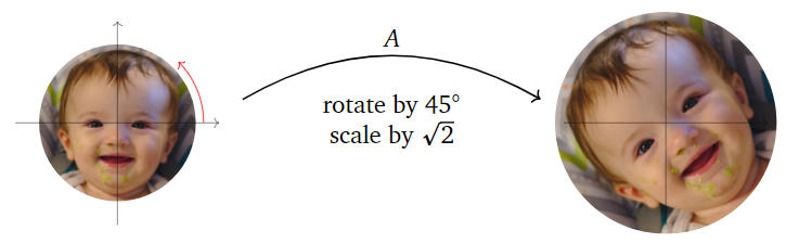
Figure $\PageIndex{4}$

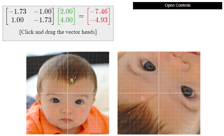
An interactive figure is included below.

Figure $\PageIndex{5}$: Multiplication by the matrix $A$ rotates the plane by $45^\circ$ and dilates by a factor of $\sqrt 2$. Move the input vector $x$ to see how the output vector $b$ changes.

Example $\PageIndex{5}$: A rotation-scaling matrix

What does the matrix

$$A = \left(\begin{array}{cc}-\sqrt{3}&-1\\1&-\sqrt{3}\end{array}\right) \nonumber$$

do geometrically?

Solution

This is a rotation-scaling matrix with $a=-\sqrt3$ and $b=1$. Therefore, it scales by a factor of $\sqrt{\det(A)}=\sqrt{3+1}=2$ and rotates counterclockwise by the angle $\theta$ in the picture:

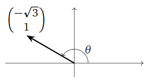
Figure $\PageIndex{6}$

To compute this angle, we do a bit of trigonometry:

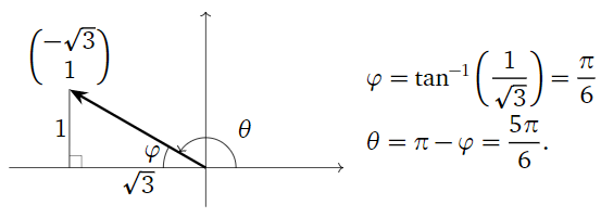
Figure $\PageIndex{7}$

Therefore, $A$ rotates counterclockwise by $5\pi/6$ and scales by a factor of $2$.

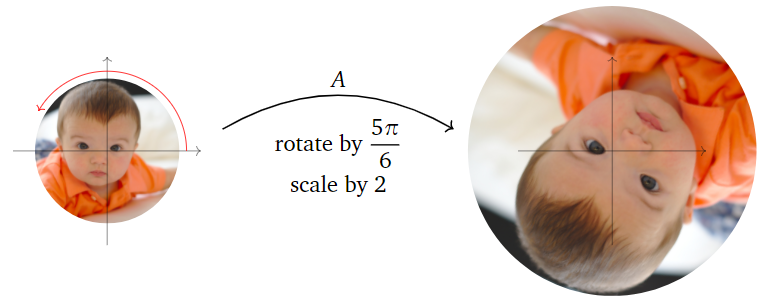
Figure $\PageIndex{8}$

An interactive figure is included below.

Figure $\PageIndex{9}$: Multiplication by the matrix $A$ rotates the plane by $5\pi/6$ and dilates by a factor of $2$. Move the input vector $x$ to see how the output vector $b$ changes.

The matrix in the second example has second column ${-\sqrt 3\choose 1}\text{,}$ which is rotated counterclockwise from the positive $x$-axis by an angle of $5\pi/6$. This rotation angle is not equal to $\tan^{-1}\bigl(1/(-\sqrt3)\bigr) = -\frac\pi 6.$ The problem is that arctan always outputs values between $-\pi/2$ and $\pi/2\text{:}$ it does not account for points in the second or third quadrants. This is why we drew a triangle and used its (positive) edge lengths to compute the angle $\varphi\text{:}$

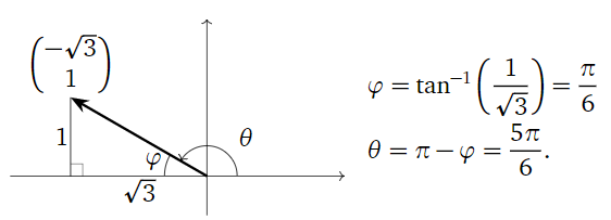
Figure $\PageIndex{10}$

Alternatively, we could have observed that ${-\sqrt 3\choose 1}$ lies in the second quadrant, so that the angle $\theta$ in question is

$$\theta = \tan^{-1}\left(\frac1{-\sqrt3}\right) + \pi. \nonumber$$

Note $\PageIndex{4}$

When finding the rotation angle of a vector ${a\choose b}\text{,}$ do not blindly compute $\tan^{-1}(b/a)\text{,}$ since this will give the wrong answer when ${a\choose b}$ is in the second or third quadrant. Instead, draw a picture.

Geometry of $2 \times 2$ Matrices with a Complex Eigenvalue

Let $A$ be a $2\times 2$ matrix with a complex, non-real eigenvalue $\lambda$. Then $A$ also has the eigenvalue $\bar\lambda\neq\lambda$. In particular, $A$ has distinct eigenvalues, so it is diagonalizable using the complex numbers. We often like to think of our matrices as describing transformations of $\mathbb{R}^n$ (as opposed to $\mathbb{C}^n$). Because of this, the following construction is useful. It gives something like a diagonalization, except that all matrices involved have real entries.

Theorem $\PageIndex{1}$: Rotation-Scaling Theorem

Let $A$ be a $2\times 2$ real matrix with a complex (non-real) eigenvalue $\lambda\text{,}$ and let $v$ be an eigenvector. Then $A = CBC^{-1}$ for

$$C = \left(\begin{array}{cc}|&| \\ \Re (v)&\Im(v) \\ |&|\end{array}\right)\quad\text{and}\quad B = \left(\begin{array}{cc}\Re(\lambda)&\Im(\lambda) \\ -\Im(\lambda)&\Re(\lambda)\end{array}\right). \nonumber$$

In particular, $A$ is similar to a rotation-scaling matrix that scales by a factor of $|\lambda| = \sqrt{\det(B)}.$

Proof

First we need to show that $\Re(v)$ and $\Im(v)$ are linearly independent, since otherwise $C$ is not invertible. If not, then there exist real numbers $x,y,$ not both equal to zero, such that $x\Re(v) + y\Im(v) = 0$. Then

$$\begin{split} (y+ix)v \amp= (y+ix)\bigl(\Re(v)+i\Im(v)\bigr) \\ \amp= y\Re(v) - x\Im(v) + \left(x\Re(v) + y\Im(v)\right)i \\ \amp= y\Re(v) - x\Im(v). \end{split} \nonumber$$

Now, $(y+ix)v$ is also an eigenvector of $A$ with eigenvalue $\lambda\text{,}$ as it is a scalar multiple of $v$. But we just showed that $(y+ix)v$ is a vector with real entries, and any real eigenvector of a real matrix has a real eigenvalue. Therefore, $\Re(v)$ and $\Im(v)$ must be linearly independent after all.

Let $\lambda = a+bi$ and $v = {x+yi\choose z+wi}$. We observe that

$$\begin{split} Av = \lambda v \amp= (a+bi)\left(\begin{array}{c}x+yi\\z+wi\end{array}\right) \\ \amp= \left(\begin{array}{c}(ax-by)+(ay+bx)i \\ (az-bw)+(aw+bz)i\end{array}\right) \\ \amp= \left(\begin{array}{c}ax-by\\az-bw\end{array}\right) + i\left(\begin{array}{c}ay+bx \\ aw+bz\end{array}\right). \end{split} \nonumber$$

On the other hand, we have

$$A\left(\left(\begin{array}{c}x\\z\end{array}\right) + i\left(\begin{array}{c}y\\w\end{array}\right)\right) = A\left(\begin{array}{c}x\\z\end{array}\right) + iA\left(\begin{array}{c}y\\w\end{array}\right) = A\Re(v) + iA\Im(v). \nonumber$$

Matching real and imaginary parts gives

$$A\Re(v) = \left(\begin{array}{c}ax-by\\az-bw\end{array}\right) \qquad A\Im(v) = \left(\begin{array}{c}ay+bx\\aw+bz\end{array}\right). \nonumber$$

Now we compute $CBC^{-1}\Re(v)$ and $CBC^{-1}\Im(v)$. Since $Ce_1 = \Re(v)$ and $Ce_2 = \Im(v)\text{,}$ we have $C^{-1}\Re(v) = e_1$ and $C^{-1}\Im(v)=e_2\text{,}$ so

$$\begin{split} CBC^{-1}\Re(v) \amp= CBe_1 = C\left(\begin{array}{c}a\\-b\end{array}\right) = a\Re(v)-b\Im(v) \\ \amp= a\left(\begin{array}{c}x\\z\end{array}\right) - b\left(\begin{array}{c}y\\w\end{array}\right) =\left(\begin{array}{c}ax-by\\az-bw\end{array}\right) = A\Re(v) \\ CBC^{-1}\Im(v) \amp= CBe_2 = C\left(\begin{array}{c}b\\a\end{array}\right) = b\Re(v)+a\Im(v) \\ \amp= b\left(\begin{array}{c}x\\z\end{array}\right) + a\left(\begin{array}{c}y\\w\end{array}\right) = \left(\begin{array}{c}ay+bx\\aw+bz\end{array}\right) = A\Im(v). \end{split} \nonumber$$

Therefore, $A\Re(v) = CBC^{-1}\Re(v)$ and $A\Im(v) = CBC^{-1}\Im(v)$.

Since $\Re(v)$ and $\Im(v)$ are linearly independent, they form a basis for $\mathbb{R}^2$. Let $w$ be any vector in $\mathbb{R}^2 \text{,}$ and write $w = c\Re(v) + d\Im(v)$. Then

$$\begin{split} Aw \amp= A\bigl(c\Re(v) + d\Im(v)\bigr) \\ \amp= cA\Re(v) + dA\Im(v) \\ \amp= cCBC^{-1}\Re(v) + dCBC^{-1}\Im(v) \\ \amp= CBC^{-1}\bigl(c\Re(v) + d\Im(v)\bigr) \\ \amp= CBC^{-1} w. \end{split} \nonumber$$

This proves that $A = CBC^{-1}$.

Here $\Re$ and $\Im$ denote the real and imaginary parts, respectively:

$$\Re(a+bi) = a \quad \Im(a+bi) = b \quad \Re\left(\begin{array}{c}x+yi\\z+wi\end{array}\right) = \left(\begin{array}{c}x\\z\end{array}\right) \quad \Im\left(\begin{array}{c}x+yi\\z+wi\end{array}\right) = \left(\begin{array}{c}y\\w\end{array}\right). \nonumber$$

The rotation-scaling matrix in question is the matrix

$$B = \left(\begin{array}{cc}a&-b\\b&a\end{array}\right)\quad\text{with}\quad a = \Re(\lambda),\; b = -\Im(\lambda). \nonumber$$

Geometrically, the rotation-scaling theorem says that a $2\times 2$ matrix with a complex eigenvalue behaves similarly to a rotation-scaling matrix. See Note 5.3.3 in Section 5.3.

One should regard Theorem $\PageIndex{1}$ as a close analogue of Theorem 5.4.1 in Section 5.4, with a rotation-scaling matrix playing the role of a diagonal matrix. Before continuing, we restate the theorem as a recipe:

Recipe: A $2\times 2$ Matrix with a Complex Eigenvalue

Let $A$ be a $2\times 2$ real matrix.

1. Compute the characteristic polynomial $$f(\lambda) = \lambda^2 - \text{Tr}(A)\lambda + \det(A), \nonumber$$ then compute its roots using the quadratic formula.
2. If the eigenvalues are complex, choose one of them, and call it $\lambda$.
3. Find a corresponding (complex) eigenvalue $v$ using the trick 3.
4. Then $A=CBC^{-1}$ for $$C = \left(\begin{array}{cc}|&| \\ \Re(v)&\Im(v) \\ |&|\end{array}\right)\quad\text{and}\quad B = \left(\begin{array}{cc}\Re(\lambda)&\Im(\lambda) \\ -\Im(\lambda)&\Re(\lambda)\end{array}\right). \nonumber$$ This scales by a factor of $|\lambda|$.

Example $\PageIndex{6}$

What does the matrix

$$A = \left(\begin{array}{cc}2&-1\\2&0\end{array}\right) \nonumber$$

do geometrically?

Solution

The eigenvalues of $A$ are

$$\lambda = \frac{\text{Tr}(A) \pm \sqrt{\text{Tr}(A)^2-4\det(A)}}2 = \frac{2\pm\sqrt{4-8}}2 = 1\pm i. \nonumber$$

We choose the eigenvalue $\lambda = 1-i$ and find a corresponding eigenvector, using the trick, note $\PageIndex{3}$:

$$A - (1-i)I_2 = \left(\begin{array}{cc}1+i&-1 \\ \star&\star\end{array}\right) \;\xrightarrow{\text{eigenvector}}\; v = \left(\begin{array}{c}1\\1+i\end{array}\right). \nonumber$$

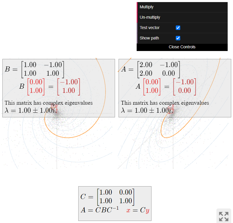
According to Theorem $\PageIndex{1}$, we have $A=CBC^{-1}$ for

$$\begin{split} C \amp= \left(\begin{array}{cc}\Re\left(\begin{array}{c}1\\1+i\end{array}\right)&\Im\left(\begin{array}{c}1\\1+i\end{array}\right)\end{array}\right) = \left(\begin{array}{cc}1&0\\1&1\end{array}\right) \\ B \amp= \left(\begin{array}{cc}\Re(\lambda)&\Im(\lambda) \\ -\Im(\lambda)&\Re(\lambda)\end{array}\right) = \left(\begin{array}{cc}1&-1\\1&1\end{array}\right). \end{split} \nonumber$$

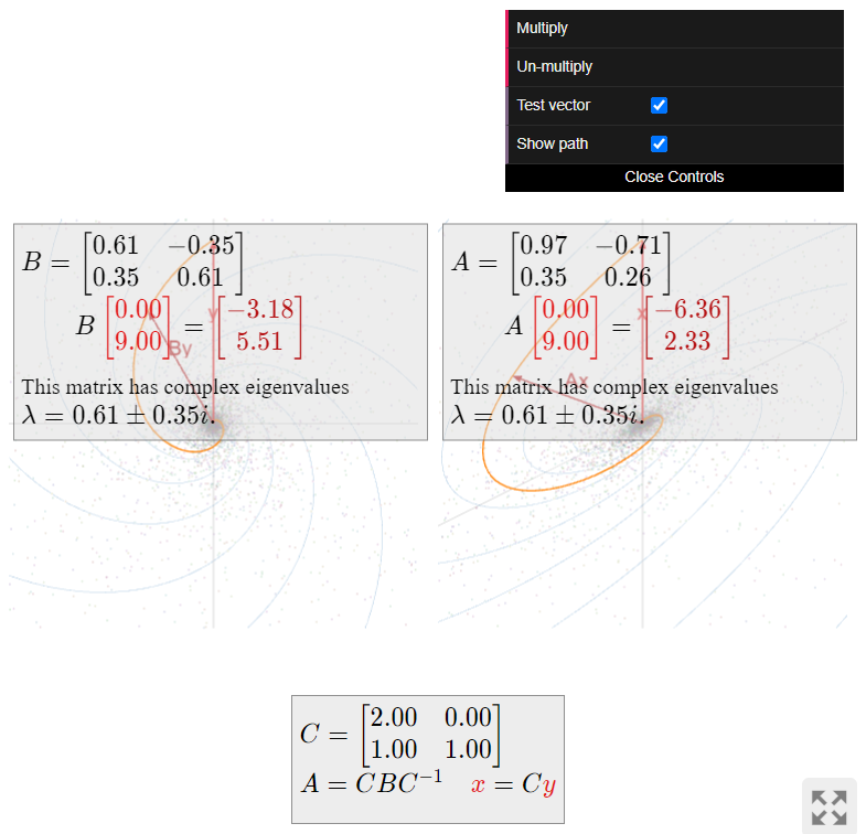
The matrix $B$ is the rotation-scaling matrix in above Example $\PageIndex{4}$: it rotates counterclockwise by an angle of $45^\circ$ and scales by a factor of $\sqrt 2$. The matrix $A$ does the same thing, but with respect to the $\Re(v),\Im(v)$-coordinate system:

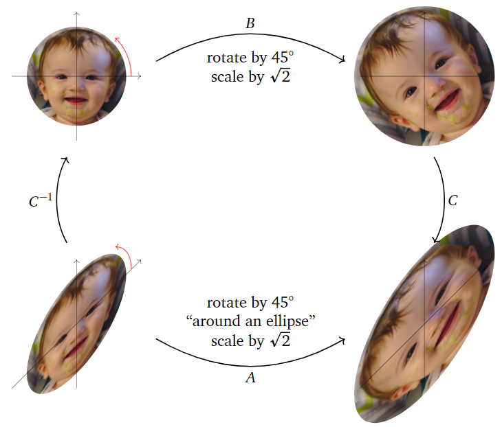
Figure $\PageIndex{11}$

To summarize:

• $B$ rotates around the circle centered at the origin and passing through $e_1$ and $e_2\text{,}$ in the direction from $e_1$ to $e_2\text{,}$ then scales by $\sqrt 2$.
• $A$ rotates around the ellipse centered at the origin and passing through $\Re(v)$ and $\Im(v)\text{,}$ in the direction from $\Re(v)$ to $\Im(v)\text{,}$ then scales by $\sqrt 2$.

The reader might want to refer back to Example 5.3.7 in Section 5.3.

Figure $\PageIndex{12}$: The geometric action of $A$ and $B$ on the plane. Click “multiply” to multiply the colored points by $B$ on the left and $A$ on the right.

If instead we had chosen $\bar\lambda = 1+i$ as our eigenvalue, then we would have found the eigenvector $\bar v = {1\choose 1-i}$. In this case we would have $A=C'B'(C')^{-1}\text{,}$ where

$$\begin{split} C' \amp= \left(\begin{array}{cc}\Re\left(\begin{array}{c}1\\1-i\end{array}\right)&\Im\left(\begin{array}{c}1\\1-i\end{array}\right)\end{array}\right) = \left(\begin{array}{cc}1&0\\1&-1\end{array}\right) \\ B' \amp= \left(\begin{array}{cc}\Re(\overline{\lambda})&\Im(\overline{\lambda}) \\ -\Im(\overline{\lambda})&\Re(\overline{\lambda})\end{array}\right) = \left(\begin{array}{cc}1&1\\-1&1\end{array}\right). \end{split} \nonumber$$

So, $A$ is also similar to a clockwise rotation by $45^\circ\text{,}$ followed by a scale by $\sqrt 2$.

Example $\PageIndex{7}$

What does the matrix

$$A = \left(\begin{array}{cc}-\sqrt{3}+1&-2\\1&-\sqrt{3}-1\end{array}\right) \nonumber$$

do geometrically?

Solution

The eigenvalues of $A$ are

$$\lambda = \frac{\text{Tr}(A) \pm \sqrt{\text{Tr}(A)^2-4\det(A)}}2 = \frac{-2\sqrt 3\pm\sqrt{12-16}}2 = -\sqrt3\pm i. \nonumber$$

We choose the eigenvalue $\lambda = -\sqrt3-i$ and find a corresponding eigenvector, using the trick, note $\PageIndex{3}$:

$$A - (-\sqrt3-i)I_2 = \left(\begin{array}{cc}1+i&-2\\ \star&\star\end{array}\right) \;\xrightarrow{\text{eigenvector}}\; v = \left(\begin{array}{c}2\\1+i\end{array}\right). \nonumber$$

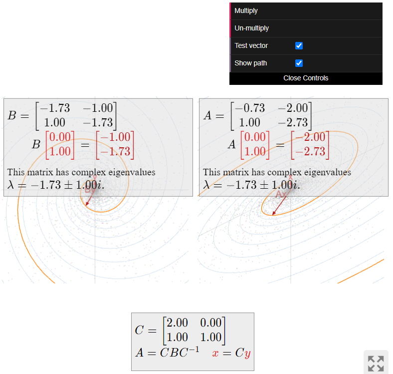
According to Theorem $\PageIndex{1}$, we have $A=CBC^{-1}$ for

$$\begin{split} C \amp= \left(\begin{array}{cc}\Re\left(\begin{array}{c}2\\1+i\end{array}\right)&\Im\left(\begin{array}{c}2\\1+i\end{array}\right)\end{array}\right) = \left(\begin{array}{cc}2&0\\1&1\end{array}\right) \\ B \amp= \left(\begin{array}{cc}\Re(\lambda)&\Im(\lambda) \\ -\Im(\lambda)&\Re(\lambda)\end{array}\right) = \left(\begin{array}{cc}-\sqrt{3}&-1\\1&-\sqrt{3}\end{array}\right). \end{split} \nonumber$$

The matrix $B$ is the rotation-scaling matrix in the above Example $\PageIndex{5}$: it rotates counterclockwise by an angle of $5\pi/6$ and scales by a factor of $2$. The matrix $A$ does the same thing, but with respect to the $\Re(v),\Im(v)$-coordinate system:

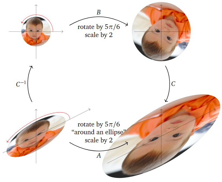
Figure $\PageIndex{13}$

To summarize:

• $B$ rotates around the circle centered at the origin and passing through $e_1$ and $e_2\text{,}$ in the direction from $e_1$ to $e_2\text{,}$ then scales by $2$.
• $A$ rotates around the ellipse centered at the origin and passing through $\Re(v)$ and $\Im(v)\text{,}$ in the direction from $\Re(v)$ to $\Im(v)\text{,}$ then scales by $2$.

The reader might want to refer back to Example 5.3.7 in Section 5.3.

Figure $\PageIndex{14}$: The geometric action of $A$ and $B$ on the plane. Click “multiply” to multiply the colored points by $B$ on the left and $A$ on the right.

If instead we had chosen $\bar\lambda = -\sqrt3-i$ as our eigenvalue, then we would have found the eigenvector $\bar v = {2\choose 1-i}$. In this case we would have $A=C'B'(C')^{-1}\text{,}$ where

$$\begin{split} C' \amp= \left(\begin{array}{cc}\Re\left(\begin{array}{c}2\\1-i\end{array}\right)&\Im\left(\begin{array}{c}2\\1-i\end{array}\right)\end{array}\right) = \left(\begin{array}{cc}2&0\\1&-1\end{array}\right) \\ B' \amp= \left(\begin{array}{cc}\Re(\overline{\lambda})&\Im(\overline{\lambda}) \\ -\Im(\overline{\lambda})&\Re(\overline{\lambda})\end{array}\right) = \left(\begin{array}{cc}-\sqrt{3}&1\\-1&-\sqrt{3}\end{array}\right). \end{split} \nonumber$$

So, $A$ is also similar to a clockwise rotation by $5\pi/6\text{,}$ followed by a scale by $2$.

We saw in the above examples that Theorem $\PageIndex{1}$ can be applied in two different ways to any given matrix: one has to choose one of the two conjugate eigenvalues to work with. Replacing $\lambda$ by $\bar\lambda$ has the effect of replacing $v$ by $\bar v\text{,}$ which just negates all imaginary parts, so we also have $A=C'B'(C')^{-1}$ for

$$C' = \left(\begin{array}{cc}|&| \\ \Re(v)&-\Im(v) \\ |&|\end{array}\right)\quad\text{and}\quad B' = \left(\begin{array}{cc}\Re(\lambda)&-\Im(\lambda) \\ \Im(\lambda)&\Re(\lambda)\end{array}\right). \nonumber$$

The matrices $B$ and $B'$ are similar to each other. The only difference between them is the direction of rotation, since ${\Re(\lambda)\choose -\Im(\lambda)}$ and ${\Re(\lambda)\choose \Im(\lambda)}$ are mirror images of each other over the $x$-axis:

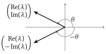
Figure $\PageIndex{15}$

The discussion that follows is closely analogous to the exposition in subsection The Geometry of Diagonalizable Matrices in Section 5.4, in which we studied the dynamics of diagonalizable $2\times 2$ matrices.

Note $\PageIndex{5}$: Dynamics of a $2\times 2$ Matrix with a Complex Eigenvalue

Let $A$ be a $2\times 2$ matrix with a complex (non-real) eigenvalue $\lambda$. By Theorem $\PageIndex{1}$, the matrix $A$ is similar to a matrix that rotates by some amount and scales by $|\lambda|$. Hence, $A$ rotates around an ellipse and scales by $|\lambda|$. There are three different cases.

$\color{Red}|\lambda| > 1\text{:}$ when the scaling factor is greater than $1\text{,}$ then vectors tend to get longer, i.e., farther from the origin. In this case, repeatedly multiplying a vector by $A$ makes the vector “spiral out”. For example,

$$A = \frac 1{\sqrt 2}\left(\begin{array}{cc}\sqrt{3}+1&-2\\1&\sqrt{3}-1\end{array}\right) \qquad \lambda = \frac{\sqrt3-i}{\sqrt 2} \qquad |\lambda| = \sqrt 2 > 1 \nonumber$$

gives rise to the following picture:

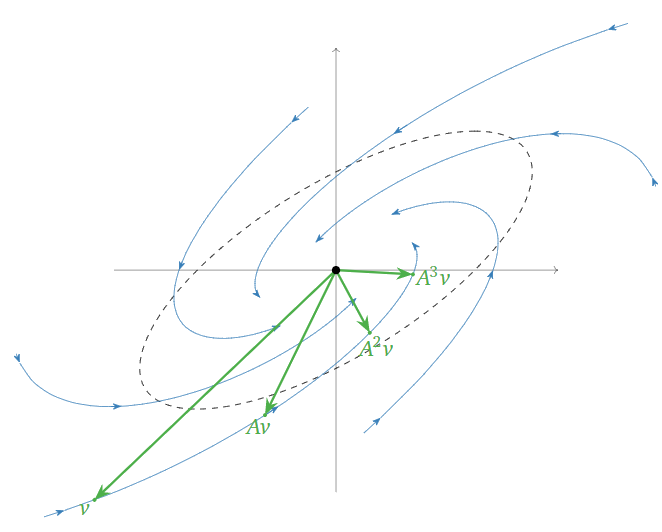
Figure $\PageIndex{16}$

$\color{Red}|\lambda| = 1\text{:}$ when the scaling factor is equal to $1\text{,}$ then vectors do not tend to get longer or shorter. In this case, repeatedly multiplying a vector by $A$ simply “rotates around an ellipse”. For example,

$$A = \frac 12\left(\begin{array}{cc}\sqrt{3}+1&-2\\1&\sqrt{3}-1\end{array}\right) \qquad \lambda = \frac{\sqrt3-i}2 \qquad |\lambda| = 1 \nonumber$$

gives rise to the following picture:

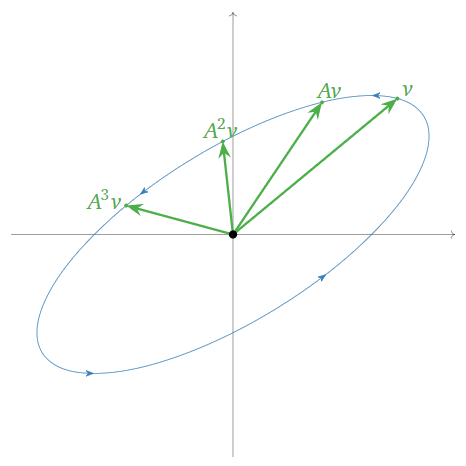
Figure $\PageIndex{17}$

$\color{Red}|\lambda| \lt 1\text{:}$ when the scaling factor is less than $1\text{,}$ then vectors tend to get shorter, i.e., closer to the origin. In this case, repeatedly multiplying a vector by $A$ makes the vector “spiral in”. For example,

$$A = \frac 1{2\sqrt 2}\left(\begin{array}{cc}\sqrt{3}+1&-2\\1&\sqrt{3}-1\end{array}\right) \qquad \lambda = \frac{\sqrt3-i}{2\sqrt 2} \qquad |\lambda| = \frac 1{\sqrt 2} \lt 1 \nonumber$$

gives rise to the following picture:

Figure $\PageIndex{18}$

Example $\PageIndex{8}$: Interactive: $|\lambda|>1$

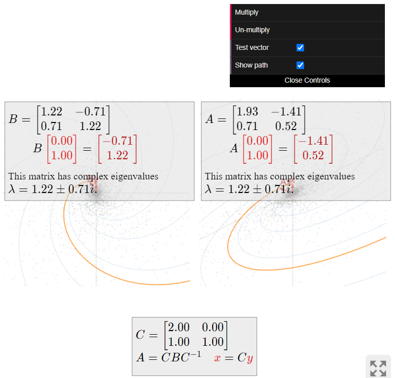
$$A = \frac 1{\sqrt 2}\left(\begin{array}{cc}\sqrt{3}+1&-2\\1&\sqrt{3}-1\end{array}\right) \qquad B = \frac 1{\sqrt 2}\left(\begin{array}{cc}\sqrt{3}&-1\\1&\sqrt{3}\end{array}\right) \qquad C = \left(\begin{array}{cc}2&0\\1&1\end{array}\right) \nonumber$$

$$\lambda = \frac{\sqrt3-i}{\sqrt 2} \qquad |\lambda| = \sqrt 2 > 1 \nonumber$$

Figure $\PageIndex{19}$: The geometric action of $A$ and $B$ on the plane. Click “multiply” to multiply the colored points by $B$ on the left and $A$ on the right.

Example $\PageIndex{9}$: Interactive: $|\lambda|=1$

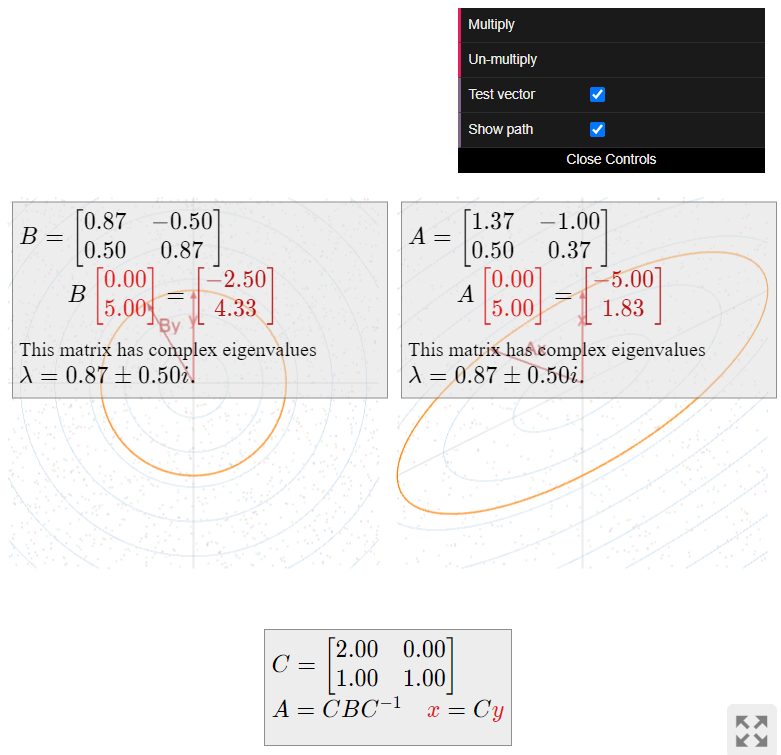
$$A = \frac 12\left(\begin{array}{cc}\sqrt{3}+1&-2\\1&\sqrt{3}-1\end{array}\right) \qquad B = \frac 12\left(\begin{array}{cc}\sqrt{3}&-1\\1&\sqrt{3}\end{array}\right) \qquad C = \left(\begin{array}{cc}2&0\\1&1\end{array}\right) \nonumber$$

$$\lambda = \frac{\sqrt3-i}2 \qquad |\lambda| = 1 \nonumber$$

Figure $\PageIndex{20}$: The geometric action of $A$ and $B$ on the plane. Click “multiply” to multiply the colored points by $B$ on the left and $A$ on the right.

Example $\PageIndex{10}$: Interactive: $|\lambda|\lt1$

$$A = \frac 1{2\sqrt 2}\left(\begin{array}{cc}\sqrt{3}+1&-2\\1&\sqrt{3}-1\end{array}\right) \qquad B = \frac 1{2\sqrt 2}\left(\begin{array}{cc}\sqrt{3}&-1\\1&\sqrt{3}\end{array}\right) \qquad C = \left(\begin{array}{cc}2&0\\1&1\end{array}\right) \nonumber$$

$$\lambda = \frac{\sqrt3-i}{2\sqrt 2} \qquad |\lambda| = \frac 1{\sqrt 2} \lt 1 \nonumber$$

Figure $\PageIndex{21}$: The geometric action of $A$ and $B$ on the plane. Click “multiply” to multiply the colored points by $B$ on the left and $A$ on the right.

Remark: Classification of $2\times 2$ matrices up to similarity

At this point, we can write down the “simplest” possible matrix which is similar to any given $2\times 2$ matrix $A$. There are four cases:

1. $A$ has two real eigenvalues $\lambda_1,\lambda_2$. In this case, $A$ is diagonalizable, so $A$ is similar to the matrix $$\left(\begin{array}{cc}\lambda_1&0\\0&\lambda_2\end{array}\right). \nonumber$$ This representation is unique up to reordering the eigenvalues.
2. $A$ has one real eigenvalue $\lambda$ of geometric multiplicity $2$. In this case, we saw in Example 5.4.20 in Section 5.4 that $A$ is equal to the matrix $$\left(\begin{array}{cc}\lambda&0\\0&\lambda\end{array}\right). \nonumber$$
3. $A$ has one real eigenvalue $\lambda$ of geometric multiplicity $1$. In this case, $A$ is not diagonalizable, and we saw in Remark: Non-diagonalizable $2\times 2$ matrices with an eigenvalue in Section 5.4 that $A$ is similar to the matrix $$\left(\begin{array}{cc}\lambda&1\\0&\lambda\end{array}\right). \nonumber$$
4. $A$ has no real eigenvalues. In this case, $A$ has a complex eigenvalue $\lambda\text{,}$ and $A$ is similar to the rotation-scaling matrix $$\left(\begin{array}{cc}\Re(\lambda)&\Im(\lambda) \\ -\Im(\lambda)&\Re(\lambda)\end{array}\right) \nonumber$$ by Theorem $\PageIndex{1}$. By Proposition $\PageIndex{1}$, the eigenvalues of a rotation-scaling matrix $\left(\begin{array}{cc}a&-b\\b&a\end{array}\right) are \(a\pm bi\text{,}$ so that two rotation-scaling matrices $\left(\begin{array}{cc}a&-b\\b&a\end{array}\right)$ and $\left(\begin{array}{cc}c&-d\\d&c\end{array}\right)$ are similar if and only if $a=c$ and $b=\pm d$.

Block Diagonalization

For matrices larger than $2\times 2\text{,}$ there is a theorem that combines Theorem 5.4.1 in Section 5.4 and Theorem $\PageIndex{1}$. It says essentially that a matrix is similar to a matrix with parts that look like a diagonal matrix, and parts that look like a rotation-scaling matrix.

Theorem $\PageIndex{2}$: Block Diagonalization Theorem

Let $A$ be a real $n\times n$ matrix. Suppose that for each (real or complex) eigenvalue, the algebraic multiplicity equals the geometric multiplicity. Then $A = CBC^{-1}\text{,}$ where $B$ and $C$ are as follows:

• The matrix $B$ is block diagonal, where the blocks are $1\times 1$ blocks containing the real eigenvalues (with their multiplicities), or $2\times 2$ blocks containing the matrices $$\left(\begin{array}{cc}\Re(\lambda)&\Im(\lambda) \\ -\Im(\lambda)&\Re(\lambda)\end{array}\right) \nonumber$$ for each non-real eigenvalue $\lambda$ (with multiplicity).
• The columns of $C$ form bases for the eigenspaces for the real eigenvectors, or come in pairs $\bigl(\,\Re(v)\;\Im(v)\,\bigr)$ for the non-real eigenvectors.

The Theorem $\PageIndex{2}$ is proved in the same way as Theorem 5.4.1 in Section 5.4 and Theorem $\PageIndex{1}$. It is best understood in the case of $3\times 3$ matrices.

Note $\PageIndex{6}$: Block Diagonalization of a $3\times 3$ Matrix with a Complex Eigenvalue

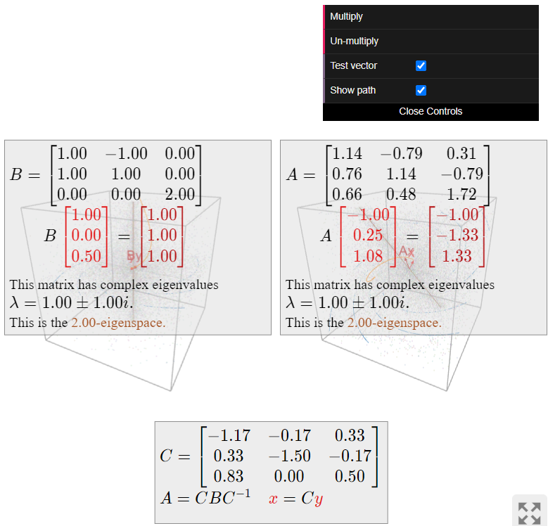
Let $A$ be a $3\times 3$ matrix with a complex eigenvalue $\lambda_1$. Then $\bar\lambda_1$ is another eigenvalue, and there is one real eigenvalue $\lambda_2$. Since there are three distinct eigenvalues, they have algebraic and geometric multiplicity one, so Theorem $\PageIndex{2}$ applies to $A$.

Let $v_1$ be a (complex) eigenvector with eigenvalue $\lambda_1\text{,}$ and let $v_2$ be a (real) eigenvector with eigenvalue $\lambda_2$. Then Theorem $\PageIndex{2}$ says that $A = CBC^{-1}$ for

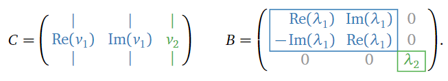
Figure $\PageIndex{22}$

Example $\PageIndex{11}$: Geometry of a $3\times 3$ matrix with a complex eigenvalue

What does the matrix

$$A = \frac 1{29}\left(\begin{array}{ccc}33&-23&9\\22&33&-23\\19&14&50\end{array}\right) \nonumber$$

do geometrically?

Solution

First we find the (real and complex) eigenvalues of $A$. We compute the characteristic polynomial using whatever method we like:

$$f(\lambda) = \det(A-\lambda I_3) = -\lambda^3 + 4\lambda^2 - 6\lambda + 4. \nonumber$$

We search for a real root using the rational root theorem. The possible rational roots are $\pm 1,\pm 2,\pm 4\text{;}$ we find $f(2) = 0\text{,}$ so that $\lambda-2$ divides $f(\lambda)$. Performing polynomial long division gives

$$f(\lambda) = -(\lambda-2)\bigl(\lambda^2-2\lambda+2\bigr). \nonumber$$

The quadratic term has roots

$$\lambda = \frac{2\pm\sqrt{4-8}}2 = 1\pm i, \nonumber$$

so that the complete list of eigenvalues is $\lambda_1 = 1-i\text{,}$ $\bar\lambda_1 = 1+i\text{,}$ and $\lambda_2 = 2$.

Now we compute some eigenvectors, starting with $\lambda_1=1-i$. We row reduce (probably with the aid of a computer):

$$A-(1-i)I_3 = \frac 1{29}\left(\begin{array}{ccc}4+29i&-23&9\\22&4+29i&-23\\19&14&21+29i\end{array}\right) \;\xrightarrow{\text{RREF}}\; \left(\begin{array}{ccc}1&0&7/5+i/5 \\ 0&1&-2/5+9i/5 \\ 0&0&0\end{array}\right). \nonumber$$

The free variable is $z\text{,}$ and the parametric form is

$$\left\{\begin{array}{ccc}x &=& -\left(\dfrac 75+\dfrac 15i\right)z\\ y &=& \left(\dfrac 25-\dfrac 95i\right)z\end{array}\right. \quad\xrightarrow[\text{eigenvector}]{z=5}\quad v_1=\left(\begin{array}{c}-7-i\\2-9i\\5\end{array}\right).\nonumber$$

For $\lambda_2=2\text{,}$ we have

$$A - 2I_3 = \frac 1{29}\left(\begin{array}{ccc}-25&-23&9\\22&-25&-23\\19&14&-8\end{array}\right) \;\xrightarrow{\text{RREF}}\; \left(\begin{array}{ccc}1&0&-2/3 \\ 0&1&1/3 \\ 0&0&0\end{array}\right). \nonumber$$

The free variable is $z\text{,}$ and the parametric form is

$$\left\{\begin{array}{rrr}x &=& \dfrac 23z \\ y &=& -\dfrac 13z \end{array}\right. \quad\xrightarrow[\text{eigenvector}]{z=3}\quad v_2=\left(\begin{array}{c}2\\-1\\3\end{array}\right).\nonumber$$

According to Theorem $\PageIndex{2}$, we have $A=CBC^{-1}$ for

$$\begin{aligned}C&=\left(\begin{array}{ccc}|&|&| \\ \Re(v_1)&\Im(v_1)&v_2 \\ |&|&|\end{array}\right)=\left(\begin{array}{ccc}-7&-1&2\\2&-9&-1\\5&0&3\end{array}\right) \\ B&=\left(\begin{array}{ccc}\Re(\lambda_1)&\Im(\lambda_1)&0 \\ -\Im(\lambda_1)&\Re(\lambda_1)&0 \\ 0&0&2\end{array}\right)=\left(\begin{array}{ccc}1&-1&0\\1&1&0\\0&0&2\end{array}\right).\end{aligned}$$

The matrix $B$ is a combination of the rotation-scaling matrix $\left(\begin{array}{cc}1&-1\\1&1\end{array}\right)$ from Example $\PageIndex{4}$, and a diagonal matrix. More specifically, $B$ acts on the $xy$-coordinates by rotating counterclockwise by $45^\circ$ and scaling by $\sqrt2\text{,}$ and it scales the $z$-coordinate by $2$. This means that points above the $xy$-plane spiral out away from the $z$-axis and move up, and points below the $xy$-plane spiral out away from the $z$-axis and move down.

The matrix $A$ does the same thing as $B\text{,}$ but with respect to the $\{\Re(v_1),\Im(v_1),v_2\}$-coordinate system. That is, $A$ acts on the $\Re(v_1),\Im(v_1)$-plane by spiraling out, and $A$ acts on the $v_2$-coordinate by scaling by a factor of $2$. See the demo below.

Figure $\PageIndex{23}$: The geometric action of $A$ and $B$ on $\mathbb{R}^3$. Click “multiply” to multiply the colored points by $B$ on the left and $A$ on the right. (We have scaled $C$ by $1/6$ so that the vectors $x$ and $y$ have roughly the same size.)