5.4: Diagonalization

\(\usepackage{macros} \newcommand{\lt}{<} \newcommand{\gt}{>} \newcommand{\amp}{&} \)

Objectives

1. Learn two main criteria for a matrix to be diagonalizable.
2. Develop a library of examples of matrices that are and are not diagonalizable.
3. Recipes: diagonalize a matrix, quickly compute powers of a matrix by diagonalization.
4. Pictures: the geometry of diagonal matrices, why a shear is not diagonalizable.
5. Theorem: the diagonalization theorem (two variants).
6. Vocabulary words: diagonalizable, algebraic multiplicity, geometric multiplicity.

Diagonal matrices are the easiest kind of matrices to understand: they just scale the coordinate directions by their diagonal entries. In Section 5.3, we saw that similar matrices behave in the same way, with respect to different coordinate systems. Therefore, if a matrix is similar to a diagonal matrix, it is also relatively easy to understand. This section is devoted to the question: “When is a matrix similar to a diagonal matrix?” This section is devoted to the question: “When is a matrix similar to a diagonal matrix?” We will see that the algebra and geometry of such a matrix is relatively easy to understand.

Diagonalizability

Before answering the above question, first we give it a name.

Definition \(\PageIndex{1}\): Diagonalizable

An \(n\times n\) matrix \(A\) is diagonalizable if it is similar to a diagonal matrix: that is, if there exists an invertible \(n\times n\) matrix \(C\) and a diagonal matrix \(D\) such that

\[ A = CDC^{-1}. \nonumber \]

Example\(\PageIndex{1}\)

Any diagonal matrix is \(D\) is diagonalizable because it is similar to itself, Proposition 5.3.1 in Section 5.3. For instance,

\[\left(\begin{array}{ccc}1&0&0\\0&2&0\\0&0&3\end{array}\right)=I_{3}\left(\begin{array}{ccc}1&0&0\\0&2&0\\0&0&3\end{array}\right)I_{3}^{-1}.\nonumber\]

Example \(\PageIndex{2}\)

Most of the examples in Section 5.3 involve diagonalizable matrices: The following are examples of diagonalizable matrices:

\[\begin{array}{lll} \left(\begin{array}{cc}-12&15\\-10&13\end{array}\right)&\begin{array}{l}\text{is diagonalizable} \\ \text{because it equals}\end{array} &\left(\begin{array}{cc}-2&3\\1&-1\end{array}\right)\left(\begin{array}{cc}3&0\\0&-2\end{array}\right)\left(\begin{array}{cc}-2&3\\1&-1\end{array}\right)^{-1} \\ \left(\begin{array}{cc}1/2&3/2\\3/2&1/2\end{array}\right)&\begin{array}{l}\text{is diagonalizable} \\ \text{because it equals}\end{array} &\left(\begin{array}{cc}1&1\\1&-1\end{array}\right)\left(\begin{array}{cc}2&0\\0&-1\end{array}\right)\left(\begin{array}{cc}1&1\\1&-1\end{array}\right)^{-1} \\ \frac{1}{5}\left(\begin{array}{cc}-8&-9\\6&13\end{array}\right)&\begin{array}{c}\text{is diagonalizable} \\ \text{because it equals}\end{array}&\frac{1}{2}\left(\begin{array}{cc}-1&-3\\2&1\end{array}\right)\left(\begin{array}{cc}2&0\\0&-1\end{array}\right)\left(\frac{1}{2}\left(\begin{array}{cc}-1&-3\\2&1\end{array}\right)\right)^{-1} \\ \left(\begin{array}{ccc}-1&0&0\\-1&0&2\\-1&1&1\end{array}\right)&\begin{array}{c}\text{is diagonalizable} \\ \text{because it equals}\end{array}&\left(\begin{array}{ccc}-1&1&0\\1&1&1\\-1&0&1\end{array}\right)\left(\begin{array}{ccc}-1&0&0\\0&-1&0\\0&0&2\end{array}\right)\left(\begin{array}{ccc}-1&1&0\\1&1&1\\-1&0&1\end{array}\right)^{-1}.\end{array}\nonumber\]

Example \(\PageIndex{3}\)

If a matrix \(A\) is diagonalizable, and if \(B\) is similar to \(A\text{,}\) then \(B\) is diagonalizable as well by Proposition 5.3.1 in Section 5.3. as well. Indeed, if \(A = CDC^{-1}\) for \(D\) diagonal, and \(B = EAE^{-1}\text{,}\) then

\[ B = EAE^{-1} = E(CDC^{-1})E^{-1} = (EC)D(EC)^{-1}, \nonumber \] so \(B\) is similar to \(D\).

Powers of Diagonalizable Matrices

Multiplying diagonal matrices together just multiplies their diagonal entries:

\[\left(\begin{array}{ccc}x_1&0&0\\0&x_2&0\\0&0&x_3\end{array}\right)\left(\begin{array}{ccc}y_1&0&0\\0&y_2&0\\0&0&y_3\end{array}\right)=\left(\begin{array}{ccc}x_1y_1&0&0\\0&x_2y_2&0\\0&0&x_3y_3\end{array}\right).\nonumber\]

Therefore, it is easy to take powers of a diagonal matrix:

\[\left(\begin{array}{ccc}x&0&0\\0&y&0\\0&0&z\end{array}\right)^{n}=\left(\begin{array}{ccc}x^n&0&0\\0&y^n&0\\0&0&z^n\end{array}\right).\nonumber\]

By Fact 5.3.1 in Section 5.3, if \(A = CDC^{-1}\) then \(A^n = CD^nC^{-1}\text{,}\) so it is also easy to take powers of diagonalizable matrices. This will be very important in applications to difference equations in Section 5.6. This is often very important in applications.

Recipe: Compute Powers of a Diagonalizable Matrix

If \(A = CDC^{-1}\text{,}\) where \(D\) is a diagonal matrix, then \(A^n = CD^nC^{-1}\text{:}\)

\[A=C\left(\begin{array}{ccc}x&0&0\\0&y&0\\0&0&z\end{array}\right)C^{-1}\quad\implies\quad A^{n}=C\left(\begin{array}{ccc}x^n&0&0\\0&y^n&0\\0&0&z^n\end{array}\right)C^{-1}.\nonumber\]

Example \(\PageIndex{4}\)

Let

\[ A = \left(\begin{array}{cc}1/2&3/2\\3/2&1/2\end{array}\right) = \left(\begin{array}{cc}1&1\\1&-1\end{array}\right) \left(\begin{array}{cc}2&0\\0&-1\end{array}\right) \left(\begin{array}{cc}1&1\\1&-1\end{array}\right)^{-1}. \nonumber \]

Find a formula for \(A^n\) in which the entries are functions of \(n\text{,}\) where \(n\) is any positive whole number.

Solution

We have

\[\begin{aligned}A^n&=\left(\begin{array}{cc}1&1\\1&-1\end{array}\right)\left(\begin{array}{cc}2&0\\0&-1\end{array}\right)^n\left(\begin{array}{cc}1&1\\1&-1\end{array}\right)^{-1} \\ &=\left(\begin{array}{cc}1&1\\1&-1\end{array}\right)\left(\begin{array}{cc}2^n&0 \\ 0&(-1)^n\end{array}\right)\frac{1}{-2}\left(\begin{array}{cc}-1&-1\\-1&1\end{array}\right) \\ &=\left(\begin{array}{cc}2^n &(-1)^n \\ 2^n&(-1)^{n+1}\end{array}\right)\frac{1}{2}\left(\begin{array}{cc}1&1\\1&-1\end{array}\right) \\ &=\frac{1}{2}\left(\begin{array}{cc} 2^n+(-1)^n &2^n +(-1)^{n+1} \\ 2^n +(-1)^{n+1} & 2^n+(-1)^n\end{array}\right),\end{aligned}\]

where we used \((-1)^{n+2}=(-1)^2(-1)^n = (-1)^n\).

A fundamental question about a matrix is whether or not it is diagonalizable. The following is the primary criterion for diagonalizability. It shows that diagonalizability is an eigenvalue problem.

Theorem \(\PageIndex{1}\): Diagonalization Theorem

An \(n\times n\) matrix \(A\) is diagonalizable if and only if \(A\) has \(n\) linearly independent eigenvectors.

In this case, \(A = CDC^{-1}\) for

\[ C = \left(\begin{array}{cccc}|&|&\quad&| \\ v_1&v_2&\cdots &v_n \\ |&|&\quad &| \end{array}\right) \qquad D = \left(\begin{array}{cccc}\lambda_{1}&0&\cdots &0 \\ 0&\lambda_2&\cdots &0 \\ \vdots &\vdots &\ddots &\vdots \\ 0&0&\cdots&\lambda_{n}\end{array}\right), \nonumber \]

where \(v_1,v_2,\ldots,v_n\) are linearly independent eigenvectors, and \(\lambda_1,\lambda_2,\ldots,\lambda_n\) are the corresponding eigenvalues, in the same order.

Proof

First suppose that \(A\) has \(n\) linearly independent eigenvectors \(v_1,v_2,\ldots,v_n\text{,}\) with eigenvalues \(\lambda_1,\lambda_2,\ldots,\lambda_n\). Define \(C\) as above, so \(C\) is invertible by Theorem 5.1.1 in Section 5.1. Let \(D = C^{-1} A C\text{,}\) so \(A = CDC^{-1}\). Multiplying by standard coordinate vectors, Fact 3.3.2 in Section 3.3, picks out the columns of \(C\text{:}\) we have \(Ce_i = v_i\text{,}\) so \(e_i = C^{-1} v_i\). We multiply by the standard coordinate vectors to find the columns of \(D\text{:}\)

\[ De_i = C^{-1} A Ce_i = C^{-1} Av_i = C^{-1}\lambda_i v_i = \lambda_iC^{-1} v_i = \lambda_ie_i. \nonumber \]

Therefore, the columns of \(D\) are multiples of the standard coordinate vectors:

\[ D = \left(\begin{array}{ccccc}\lambda_{1}&0&\cdots &0&0\\ 0&\lambda_{2}&\cdots &0&0 \\ \vdots &\vdots &\ddots&\vdots&\vdots \\ 0&0&\cdots&\lambda_{n-1}&0 \\ 0&0&\cdots &0&\lambda_{n}\end{array}\right). \nonumber \]

Now suppose that \(A = CDC^{-1}\text{,}\) where \(C\) has columns \(v_1,v_2,\ldots,v_n\text{,}\) and \(D\) is diagonal with diagonal entries \(\lambda_1,\lambda_2,\ldots,\lambda_n\). Since \(C\) is invertible, its columns are linearly independent. We have to show that \(v_i\) is an eigenvector of \(A\) with eigenvalue \(\lambda_i\). We know that the standard coordinate vector \(e_i\) is an eigenvector of \(D\) with eigenvalue \(\lambda_i\text{,}\) so:

\[ Av_i = CDC^{-1} v_i = CDe_i = C\lambda_ie_i = \lambda_iCe_i = \lambda_i v_i. \nonumber \]

By Fact 5.1.1 in Section 5.1, if an \(n\times n\) matrix \(A\) has \(n\) distinct eigenvalues \(\lambda_1,\lambda_2,\ldots,\lambda_n\text{,}\) then a choice of corresponding eigenvectors \(v_1,v_2,\ldots,v_n\) is automatically linearly independent.

Note \(\PageIndex{1}\)

An \(n\times n\) matrix with \(n\) distinct eigenvalues is diagonalizable.

Example \(\PageIndex{5}\): Easy Example

Apply Theorem \(\PageIndex{1}\) to the matrix

\[ A = \left(\begin{array}{ccc}1&0&0\\0&2&0\\0&0&3\end{array}\right). \nonumber \]

Solution

This diagonal matrix is in particular upper-triangular, so its eigenvalues are the diagonal entries \(1,2,3\). The standard coordinate vectors are eigenvalues of a diagonal matrix:

\[\left(\begin{array}{ccc}1&0&0\\0&2&0\\0&0&3\end{array}\right)\left(\begin{array}{c}1\\0\\0\end{array}\right)=1\cdot\left(\begin{array}{c}1\\0\\0\end{array}\right)\quad\left(\begin{array}{ccc}1&0&0\\0&2&0\\0&0&3\end{array}\right)\left(\begin{array}{c}0\\1\\0\end{array}\right)=2\cdot\left(\begin{array}{c}0\\1\\0\end{array}\right)\nonumber\]

\[\left(\begin{array}{ccc}1&0&0\\0&2&0\\0&0&3\end{array}\right)\left(\begin{array}{c}0\\0\\1\end{array}\right)=3\cdot\left(\begin{array}{c}0\\0\\1\end{array}\right).\nonumber\]

Therefore, the diagonalization theorem says that \(A=CDC^{-1}\text{,}\) where the columns of \(C\) are the standard coordinate vectors, and the \(D\) is the diagonal matrix with entries \(1,2,3\text{:}\)

\[\left(\begin{array}{ccc}1&0&0\\0&2&0\\0&0&3\end{array}\right)=\left(\begin{array}{ccc}1&0&0\\0&1&0\\0&0&1\end{array}\right)\left(\begin{array}{ccc}1&0&0\\0&2&0\\0&0&3\end{array}\right)\left(\begin{array}{ccc}1&0&0\\0&1&0\\0&0&1\end{array}\right)^{-1}.\nonumber\]

This just tells us that \(A\) is similar to itself.

Actually, the diagonalization theorem is not completely trivial even for diagonal matrices. If we put our eigenvalues in the order \(3,2,1\text{,}\) then the corresponding eigenvectors are \(e_3,e_2,e_1\text{,}\) so we also have that \(A = C'D'(C')^{-1}\text{,}\) where \(C'\) is the matrix with columns \(e_3,e_2,e_1\text{,}\) and \(D'\) is the diagonal matrix with entries \(3,2,1\text{:}\)

\[\left(\begin{array}{ccc}1&0&0\\0&2&0\\0&0&3\end{array}\right)=\left(\begin{array}{ccc}0&0&1\\0&1&0\\1&0&0\end{array}\right)\left(\begin{array}{ccc}3&0&0\\0&2&0\\0&0&1\end{array}\right)\left(\begin{array}{ccc}0&0&1\\0&1&0\\1&0&0\end{array}\right)^{-1}.\nonumber\]

In particular, the matrices

\[\left(\begin{array}{ccc}1&0&0\\0&2&0\\0&0&3\end{array}\right)\quad\text{and}\quad\left(\begin{array}{ccc}3&0&0\\0&2&0\\0&0&1\end{array}\right)\nonumber\]

are similar to each other.

Note \(\PageIndex{2}\): Non-Uniqueness of Diagonalization

We saw in the above example that changing the order of the eigenvalues and eigenvectors produces a different diagonalization of the same matrix. There are generally many different ways to diagonalize a matrix, corresponding to different orderings of the eigenvalues of that matrix. The important thing is that the eigenvalues and eigenvectors have to be listed in the same order.

\[\begin{aligned}A&=\left(\begin{array}{ccc}|&|&|\\ v_1&v_2&v_3\\|&|&|\end{array}\right)\left(\begin{array}{ccc}\lambda_1&0&0\\0&\lambda_2&0\\0&0&\lambda_3\end{array}\right)\left(\begin{array}{ccc}|&|&|\\v_1&v_2&v_3\\ |&|&|\end{array}\right)^{-1} \\ &=\left(\begin{array}{ccc}|&|&|\\v_3&v_2&v_1 \\ |&|&|\end{array}\right)\left(\begin{array}{ccc}\lambda_3&0&0 \\ 0&\lambda_2&0 \\ 0&0&\lambda_1\end{array}\right) \left(\begin{array}{ccc}|&|&|\\v_3&v_2&v_1\\ |&|&|\end{array}\right)^{-1}.\end{aligned}\]

There are other ways of finding different diagonalizations of the same matrix. For instance, you can scale one of the eigenvectors by a constant \(c\text{:}\)

\[\begin{aligned}A&=\left(\begin{array}{ccc}|&|&|\\ v_1&v_2&v_3\\|&|&|\end{array}\right)\left(\begin{array}{ccc}\lambda_1&0&0\\0&\lambda_2&0\\0&0&\lambda_3\end{array}\right)\left(\begin{array}{ccc}|&|&|\\v_1&v_2&v_3\\ |&|&|\end{array}\right)^{-1} \\ &=\left(\begin{array}{ccc}|&|&|\\cv_1&v_2&v_3 \\ |&|&|\end{array}\right)\left(\begin{array}{ccc}\lambda_1&0&0 \\ 0&\lambda_2&0 \\ 0&0&\lambda_3\end{array}\right) \left(\begin{array}{ccc}|&|&|\\cv_1&v_2&v_3\\ |&|&|\end{array}\right)^{-1}.\end{aligned}\]

you can find a different basis entirely for an eigenspace of dimension at least \(2\text{,}\) etc.

Example \(\PageIndex{6}\): A diagonalizable \(2\times 2\) matrix

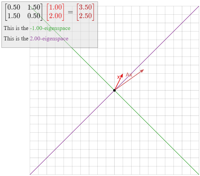
Diagonalize the matrix

\[ A = \left(\begin{array}{cc}1/2&3/2\\3/2&1/2\end{array}\right). \nonumber \]

Solution

We need to find the eigenvalues and eigenvectors of \(A\). First we compute the characteristic polynomial:

\[ f(\lambda) = \lambda^2-\text{Tr}(A)\lambda + \det(A) = \lambda^2-\lambda-2 = (\lambda+1)(\lambda-2). \nonumber \]

Therefore, the eigenvalues are \(-1\) and \(2\). We need to compute eigenvectors for each eigenvalue. We start with \(\lambda_1 = -1\text{:}\)

\[ (A + 1I_2)v = 0 \iff \left(\begin{array}{cc}3/2&3/2\\3/2&3/2\end{array}\right)v = 0 \;\xrightarrow{\text{RREF}}\; \left(\begin{array}{cc}1&1\\0&0\end{array}\right)v = 0. \nonumber \]

The parametric form is \(x = -y\text{,}\) so \(v_1 = {-1\choose 1}\) is an eigenvector with eigenvalue \(\lambda_1\). Now we find an eigenvector with eigenvalue \(\lambda_2 = 2\text{:}\)

\[ (A-2I_2)v = 0 \iff \left(\begin{array}{cc}-3/2&3/2\\3/2&-3/2\end{array}\right)v = 0 \;\xrightarrow{\text{RREF}}\; \left(\begin{array}{cc}1&-1\\0&0\end{array}\right)v = 0. \nonumber \]

The parametric form is \(x = y\text{,}\) so \(v_2 = {1\choose 1}\) is an eigenvector with eigenvalue \(2\).

The eigenvectors \(v_1,v_2\) are linearly independent, so Theorem \(\PageIndex{1}\) says that

\[ A = CDC^{-1} \qquad\text{for}\qquad C = \left(\begin{array}{cc}-1&1\\1&1\end{array}\right) \qquad D = \left(\begin{array}{cc}-1&0\\0&2\end{array}\right). \nonumber \]

Alternatively, if we choose \(2\) as our first eigenvalue, then

\[ A = C'D'(C')^{-1} \qquad\text{for}\qquad C' =\left(\begin{array}{cc}1&-1\\1&1\end{array}\right) \qquad D' = \left(\begin{array}{cc}2&0\\0&-1\end{array}\right). \nonumber \]

Figure \(\PageIndex{1}\): The green line is the \(-1\)-eigenspace of \(A\text{,}\) and the violet line is the \(2\)-eigenspace. There are two linearly independent (noncollinear) eigenvectors visible in the picture: choose any nonzero vector on the green line, and any nonzero vector on the violet line.

Example \(\PageIndex{7}\): A diagonalizable \(2\times 2\) matrix with a zero eigenvector

Diagonalize the matrix

\[ A =\left(\begin{array}{cc}2/3&-4/3\\-2/3&4/3\end{array}\right). \nonumber \]

Solution

We need to find the eigenvalues and eigenvectors of \(A\). First we compute the characteristic polynomial:

\[ f(\lambda) = \lambda^2-\text{Tr}(A)\lambda + \det(A) = \lambda^2 -2\lambda = \lambda(\lambda-2). \nonumber \]

Therefore, the eigenvalues are \(0\) and \(2\). We need to compute eigenvectors for each eigenvalue. We start with \(\lambda_1 = 0\text{:}\)

\[ (A - 0I_2)v = 0 \iff \left(\begin{array}{cc}2/3&-4/3\\-2/3&4/3\end{array}\right)v = 0 \;\xrightarrow{\text{RREF}}\; \left(\begin{array}{cc}1&-2\\0&0\end{array}\right)v = 0. \nonumber \]

The parametric form is \(x = 2y\text{,}\) so \(v_1 = {2\choose 1}\) is an eigenvector with eigenvalue \(\lambda_1\). Now we find an eigenvector with eigenvalue \(\lambda_2 = 2\text{:}\)

\[ (A-2I_2)v = 0 \iff \left(\begin{array}{cc}-4/3&-4/3\\-2/3&-2/3\end{array}\right)v = 0 \;\xrightarrow{\text{RREF}}\; \left(\begin{array}{cc}1&1\\0&0\end{array}\right)v = 0. \nonumber \]

The parametric form is \(x = -y\text{,}\) so \(v_2 = {1\choose-1}\) is an eigenvector with eigenvalue \(2\).

The eigenvectors \(v_1,v_2\) are linearly independent, so the Theorem \(\PageIndex{1}\) says that

\[ A = CDC^{-1} \qquad\text{for}\qquad C =\left(\begin{array}{cc}2&1\\1&-1\end{array}\right) \qquad D = \left(\begin{array}{cc}0&0\\0&2\end{array}\right). \nonumber \]

Alternatively, if we choose \(2\) as our first eigenvalue, then

\[ A = C'D'(C')^{-1} \qquad\text{for}\qquad C' = \left(\begin{array}{cc}1&2\\-1&1\end{array}\right) \qquad D' = \left(\begin{array}{cc}2&0\\0&0\end{array}\right). \nonumber \]

In the above example, the (non-invertible) matrix \(A = \frac 13\left(\begin{array}{cc}2&-4\\-2&4\end{array}\right)\) is similar to the diagonal matrix \(D = \left(\begin{array}{cc}0&0\\0&2\end{array}\right).\) Since \(A\) is not invertible, zero is an eigenvalue by the invertible matrix theorem, Theorem 5.1.1 in Section 5.1, so one of the diagonal entries of \(D\) is necessarily zero. Also see Example \(\PageIndex{10}\) below.

Example \(\PageIndex{8}\): A diagonalizable \(3\times 3\) matrix

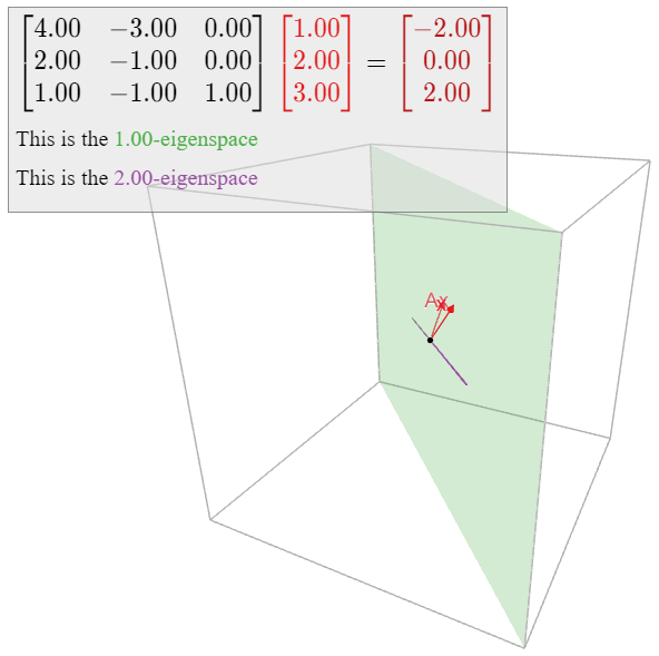
Diagonalize the matrix

\[ A = \left(\begin{array}{ccc}4&-3&0\\2&-1&0\\1&-1&1\end{array}\right). \nonumber \]

Solution

We need to find the eigenvalues and eigenvectors of \(A\). First we compute the characteristic polynomial by expanding cofactors along the third column:

\[ \begin{split} f(\lambda) \amp= \det(A-\lambda I_3) = (1-\lambda)\det\left(\left(\begin{array}{cc}4&-3\\2&-1\end{array}\right) - \lambda I_2\right) \\ \amp= (1-\lambda)(\lambda^2 - 3\lambda + 2) = -(\lambda-1)^2(\lambda-2). \end{split} \nonumber \]

Therefore, the eigenvalues are \(1\) and \(2\). We need to compute eigenvectors for each eigenvalue. We start with \(\lambda_1 = 1\text{:}\)

\[ (A-I_3)v = 0 \iff \left(\begin{array}{ccc}3&-3&0\\2&-2&0\\1&-1&0\end{array}\right)v = 0 \;\xrightarrow{\text{RREF}}\; \left(\begin{array}{ccc}1&-1&0\\0&0&0\\0&0&0\end{array}\right)v = 0. \nonumber \]

The parametric vector form is

\[\left\{\begin{array}{rrr}x&=&y \\ y&=&y \\ z&=&z \end{array}\right.\implies\left(\begin{array}{c}x\\y\\z\end{array}\right)+y\left(\begin{array}{c}1\\1\\0\end{array}\right)+z\left(\begin{array}{c}0\\0\\1\end{array}\right).\nonumber\]

Hence a basis for the \(1\)-eigenspace is

\[\mathcal{B}_{1}=\{v_1,\:v_2\}\quad\text{where}\quad v_1=\left(\begin{array}{c}1\\1\\0\end{array}\right),\quad v_2=\left(\begin{array}{c}0\\0\\1\end{array}\right).\nonumber\]

Now we compute the eigenspace for \(\lambda_2 = 2\text{:}\)

\[ (A-2I_3)v = 0 \iff \left(\begin{array}{ccc}2&-3&0\\2&-3&0\\1&-1&-1\end{array}\right)v = 0 \;\xrightarrow{\text{RREF}}\; \left(\begin{array}{ccc}1&0&-3\\0&1&-2\\0&0&0\end{array}\right)v = 0 \nonumber \]

The parametric form is \(x = 3z, y = 2z\text{,}\) so an eigenvector with eigenvalue \(2\) is

\[ v_3 = \left(\begin{array}{c}3\\2\\1\end{array}\right). \nonumber \]

The eigenvectors \(v_1,v_2,v_3\) are linearly independent: \(v_1,v_2\) form a basis for the \(1\)-eigenspace, and \(v_3\) is not contained in the \(1\)-eigenspace because its eigenvalue is \(2\). Therefore, Theorem \(\PageIndex{1}\) says that

\[ A = CDC^{-1} \qquad\text{for}\qquad C = \left(\begin{array}{ccc}1&0&3\\1&0&2\\0&1&1\end{array}\right) \qquad D = \left(\begin{array}{ccc}1&0&0\\0&1&0\\0&0&2\end{array}\right). \nonumber \]

Figure \(\PageIndex{2}\): The green plane is the \(1\)-eigenspace of \(A\text{,}\) and the violet line is the \(2\)-eigenspace. There are three linearly independent eigenvectors visible in the picture: choose any two noncollinear vectors on the green plane, and any nonzero vector on the violet line.

Here is the procedure we used in the above examples.

Recipe: Diagonalization

Let \(A\) be an \(n\times n\) matrix. To diagonalize \(A\text{:}\)

1. Find the eigenvalues of \(A\) using the characteristic polynomial.
2. For each eigenvalue \(\lambda\) of \(A\text{,}\) compute a basis \(\mathcal{B}_\lambda\) for the \(\lambda\)-eigenspace.
3. If there are fewer than \(n\) total vectors in all of the eigenspace bases \(B_\lambda\text{,}\) then the matrix is not diagonalizable.
4. Otherwise, the \(n\) vectors \(v_1,v_2,\ldots,v_n\) in the eigenspace bases are linearly independent, and \(A = CDC^{-1}\) for \[C=\left(\begin{array}{cccc}|&|&\quad &| \\ v_1&v_2&\cdots &v_n \\ |&|&\quad &|\end{array}\right)\quad\text{and}\quad D=\left(\begin{array}{cccc}\lambda_1&0&\cdots &0 \\ 0&\lambda_2&\cdots &0 \\ \vdots&\vdots &\ddots&\vdots \\ 0&0&\cdots &\lambda_n\end{array}\right),\nonumber\] where \(\lambda_i\) is the eigenvalue for \(v_i\).

We will justify the linear independence assertion in part 4 in the proof of Theorem \(\PageIndex{3}\) below.

Example \(\PageIndex{9}\): A shear is not diagonalizable

Let

\[ A = \left(\begin{array}{cc}1&1\\0&1\end{array}\right), \nonumber \]

so \(T(x) = Ax\) is a shear, Example 3.1.8 in Section 3.1. The characteristic polynomial of \(A\) is \(f(\lambda) = (\lambda-1)^2\text{,}\) so the only eigenvalue of \(A\) is \(1\). We compute the \(1\)-eigenspace:

\[ (A - I_2)v = 0 \iff \left(\begin{array}{cc}0&1\\0&0\end{array}\right)\left(\begin{array}{c}x\\y\end{array}\right)= 0 \iff y = 0. \nonumber \]

In other words, the \(1\)-eigenspace is exactly the \(x\)-axis, so all of the eigenvectors of \(A\) lie on the \(x\)-axis. It follows that \(A\) does not admit two linearly independent eigenvectors, so by Theorem \(\PageIndex{1}\), it is not diagonalizable.

In Example 5.1.8 in Section 5.1, we studied the eigenvalues of a shear geometrically; we reproduce the interactive demo here.

Figure \(\PageIndex{3}\): All eigenvectors of a shear lie on the \(x\)-axis.

Example \(\PageIndex{10}\): A projection is diagonalizable

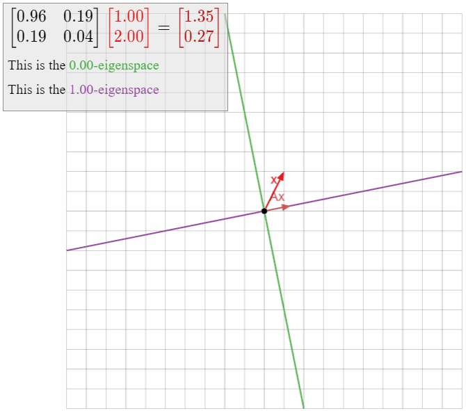
Let \(L\) be a line through the origin in \(\mathbb{R}^2 \text{,}\) and define \(T\colon\mathbb{R}^2 \to\mathbb{R}^2 \) to be the transformation that sends a vector \(x\) to the closest point on \(L\) to \(x\text{,}\) as in the picture below.

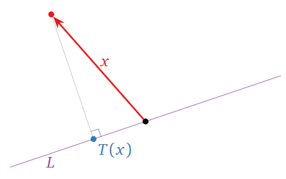
Figure \(\PageIndex{4}\)

This is an example of an orthogonal projection. We will see in Section 6.3 that \(T\) is a linear transformation; let \(A\) be the matrix for \(T\). Any vector on \(L\) is not moved by \(T\) because it is the closest point on \(L\) to itself: hence it is an eigenvector of \(A\) with eigenvalue \(1\). Let \(L^\perp\) be the line perpendicular to \(L\) and passing through the origin. Any vector \(x\) on \(L^\perp\) is closest to the zero vector on \(L\text{,}\) so a (nonzero) such vector is an eigenvector of \(A\) with eigenvalue \(0\). (See Example 5.1.5 in Section 5.1 for a special case.) Since \(A\) has two distinct eigenvalues, it is diagonalizable; in fact, we know from Theorem \(\PageIndex{1}\) that \(A\) is similar to the matrix \(\left(\begin{array}{cc}1&0\\0&0\end{array}\right)\).

Note that we never had to do any algebra! We know that \(A\) is diagonalizable for geometric reasons.

Figure \(\PageIndex{5}\): The line \(L\) (violet) is the \(1\)-eigenspace of \(A\text{,}\) and \(L^\perp\) (green) is the \(0\)-eigenspace. Since there are linearly independent eigenvectors, we know that \(A\) is diagonalizable.

Example \(\PageIndex{11}\): A non-diagonalizable \(3\times 3\) matrix

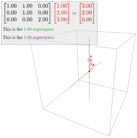
Let

\[ A =\left(\begin{array}{ccc}1&1&0\\0&1&0\\0&0&2\end{array}\right). \nonumber \]

The characteristic polynomial of \(A\) is \(f(\lambda) = -(\lambda-1)^2(\lambda-2)\text{,}\) so the eigenvalues of \(A\) are \(1\) and \(2\). We compute the \(1\)-eigenspace:

\[ (A - I_3)v = 0 \iff \left(\begin{array}{ccc}0&1&0\\0&0&0\\0&0&2\end{array}\right)\left(\begin{array}{c}x\\y\\z\end{array}\right) = 0 \iff y = z = 0. \nonumber \]

In other words, the \(1\)-eigenspace is the \(x\)-axis. Similarly,

\[ (A - 2I_3)v = 0 \iff \left(\begin{array}{ccc}-1&1&0\\0&-1&0\\0&0&0\end{array}\right)\left(\begin{array}{c}x\\y\\z\end{array}\right) = 0 \iff x = y = 0, \nonumber \]

so the \(2\)-eigenspace is the \(z\)-axis. In particular, all eigenvectors of \(A\) lie on the \(xz\)-plane, so there do not exist three linearly independent eigenvectors of \(A\). By Theorem \(\PageIndex{1}\), the matrix \(A\) is not diagonalizable.

Notice that \(A\) contains a \(2\times 2\) block on its diagonal that looks like a shear:

\[A=\left(\begin{array}{ccc}\color{Red}{1}&\color{Red}{1}&\color{black}{0}\\ \color{Red}{0}&\color{Red}{1}&\color{black}{0} \\ 0&0&2\end{array}\right).\nonumber\]

This makes one suspect that such a matrix is not diagonalizable.

Figure \(\PageIndex{6}\): All eigenvectors of \(A\) lie on the \(x\)- and \(z\)-axes.

Example \(\PageIndex{12}\): A rotation matrix

Let

\[ A = \left(\begin{array}{cc}0&-1\\1&0\end{array}\right), \nonumber \]

so \(T(x) = Ax\) is the linear transformation that rotates counterclockwise by \(90^\circ\). We saw in Example 5.1.9 in Section 5.1 that \(A\) does not have any eigenvectors at all. It follows that \(A\) is not diagonalizable.

Figure \(\PageIndex{7}\): This rotation matrix has no eigenvectors.

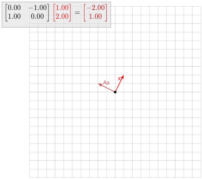
The characteristic polynomial of \(A\) is \(f(\lambda) = \lambda^2+1\text{,}\) which of course does not have any real roots. If we allow complex numbers, however, then \(f\) has two roots, namely, \(\pm i\text{,}\) where \(i = \sqrt{-1}\). Hence the matrix is diagonalizable if we allow ourselves to use complex numbers. We will treat this topic in detail in Section 5.5.

The following point is often a source of confusion.

Note \(\PageIndex{3}\): Diagonalizability has nothing to do with invertibility

Of the following matrices, the first is diagonalizable and invertible, the second is diagonalizable but not invertible, the third is invertible but not diagonalizable, and the fourth is neither invertible nor diagonalizable, as the reader can verify:

\[\left(\begin{array}{cc}1&0\\0&1\end{array}\right)\quad\left(\begin{array}{cc}1&0\\0&0\end{array}\right)\quad\left(\begin{array}{cc}1&1\\0&1\end{array}\right)\quad\left(\begin{array}{cc}0&1\\0&0\end{array}\right).\nonumber\]

Remark: Non-diagonalizable \(2\times 2\) matrices with an eigenvalue

As in the above Example \(\PageIndex{9}\), one can check that the matrix

\[ A_\lambda = \left(\begin{array}{cc}\lambda&1\\0&\lambda\end{array}\right) \nonumber \]

is not diagonalizable for any number \(\lambda\). We claim that any non-diagonalizable \(2\times 2\) matrix \(B\) with a real eigenvalue \(\lambda\) is similar to \(A_\lambda\). Therefore, up to similarity, these are the only such examples.

To prove this, let \(B\) be such a matrix. Let \(v_1\) be an eigenvector with eigenvalue \(\lambda\text{,}\) and let \(v_2\) be any vector in \(\mathbb{R}^2 \) that is not collinear with \(v_1\text{,}\) so that \(\{v_1,v_2\}\) forms a basis for \(\mathbb{R}^2 \). Let \(C\) be the matrix with columns \(v_1,v_2\text{,}\) and consider \(A = C^{-1} BC\). We have \(Ce_1=v_1\) and \(Ce_2=v_2\text{,}\) so \(C^{-1} v_1=e_1\) and \(C^{-1} v_2=e_2\). We can compute the first column of \(A\) as follows:

\[ Ae_1 = C^{-1} BC e_1 = C^{-1} Bv_1 = C^{-1}\lambda v_1 = \lambda C^{-1} v_1 = \lambda e_1. \nonumber \]

Therefore, \(A\) has the form

\[ A = \left(\begin{array}{cc}\lambda&b\\0&d\end{array}\right). \nonumber \]

Since \(A\) is similar to \(B\text{,}\) it also has only one eigenvalue \(\lambda\text{;}\) since \(A\) is upper-triangular, this implies \(d=\lambda\text{,}\) so

\[ A = \left(\begin{array}{cc}\lambda&b\\0&\lambda\end{array}\right). \nonumber \]

As \(B\) is not diagonalizable, we know \(A\) is not diagonal (\(B\) is similar to \(A\)), so \(b\neq 0\). Now we observe that

\[\left(\begin{array}{cc}1/b&0\\0&1\end{array}\right)\left(\begin{array}{cc}\lambda&b\\0&\lambda\end{array}\right)\left(\begin{array}{cc}1/b&0\\0&1\end{array}\right)^{-1}=\left(\begin{array}{cc}\lambda /b&1 \\ 0&\lambda\end{array}\right)\left(\begin{array}{cc}b&0\\0&1\end{array}\right)=\left(\begin{array}{cc}\lambda&1 \\ 0&\lambda\end{array}\right)=A_{\lambda}.\nonumber\]

We have shown that \(B\) is similar to \(A\text{,}\) which is similar to \(A_\lambda\text{,}\) so \(B\) is similar to \(A_\lambda\) by the transitivity property, Proposition 5.3.1 in Section 5.3, of similar matrices. 

The Geometry of Diagonalizable Matrices

A diagonal matrix is easy to understand geometrically, as it just scales the coordinate axes:

\[\left(\begin{array}{ccc}1&0&0\\0&2&0\\0&0&3\end{array}\right)\left(\begin{array}{c}1\\0\\0\end{array}\right)=1\cdot\left(\begin{array}{c}1\\0\\0\end{array}\right)\quad\left(\begin{array}{ccc}1&0&0\\0&2&0\\0&0&3\end{array}\right)\left(\begin{array}{c}0\\1\\0\end{array}\right)=2\cdot\left(\begin{array}{c}0\\1\\0\end{array}\right)\nonumber\]

\[\left(\begin{array}{ccc}1&0&0\\0&2&0\\0&0&3\end{array}\right)\left(\begin{array}{c}0\\0\\1\end{array}\right)=3\cdot\left(\begin{array}{c}0\\0\\1\end{array}\right).\nonumber\]

Therefore, we know from Section 5.3 that a diagonalizable matrix simply scales the “axes” with respect to a different coordinate system. Indeed, if \(v_1,v_2,\ldots,v_n\) are linearly independent eigenvectors of an \(n\times n\) matrix \(A\text{,}\) then \(A\) scales the \(v_i\)-direction by the eigenvalue \(\lambda_i\).

In the following examples, we visualize the action of a diagonalizable matrix \(A\) in terms of its dynamics. In other words, we start with a collection of vectors (drawn as points), and we see where they move when we multiply them by \(A\) repeatedly.

Example \(\PageIndex{13}\): Eigenvalues \(|\lambda_1| > 1,\,|\lambda_2|\lt1\)

Describe how the matrix

\[ A = \frac{1}{10}\left(\begin{array}{cc}11&6\\9&14\end{array}\right) \nonumber \]

acts on the plane.

Solution

First we diagonalize \(A\). The characteristic polynomial is

\[ f(\lambda) = \lambda^2 - \text{Tr}(A)\lambda + \det(A) = \lambda^2 - \frac 52\lambda + 1 = (\lambda - 2)\left(\lambda - \frac 12\right). \nonumber \]

We compute the \(2\)-eigenspace:

\[ (A-2I_3)v = 0 \iff \frac 1{10}\left(\begin{array}{cc}-9&6\\9&-6\end{array}\right)v = 0 \;\xrightarrow{\text{RREF}}\; \left(\begin{array}{cc}1&-2/3\\0&0\end{array}\right)v = 0. \nonumber \]

The parametric form of this equation is \(x = 2/3y\text{,}\) so one eigenvector is \(v_1 = {2/3\choose 1}\). For the \(1/2\)-eigenspace, we have:

\[ \left(A-\frac 12I_3\right)v = 0 \iff \frac 1{10}\left(\begin{array}{cc}6&6\\9&9\end{array}\right)v = 0 \;\xrightarrow{\text{RREF}}\; \left(\begin{array}{cc}1&1\\0&0\end{array}\right)v = 0. \nonumber \]

The parametric form of this equation is \(x = -y\text{,}\) so an eigenvector is \(v_2 = {-1\choose 1}\). It follows that \(A = CDC^{-1}\text{,}\) where

\[ C = \left(\begin{array}{cc}2/3&-1 \\ 1&1\end{array}\right) \qquad D = \left(\begin{array}{cc}2&0\\0&1/2\end{array}\right). \nonumber \]

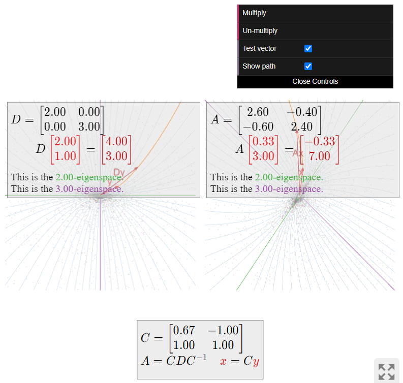
The diagonal matrix \(D\) scales the \(x\)-coordinate by \(2\) and the \(y\)-coordinate by \(1/2\). Therefore, it moves vectors closer to the \(x\)-axis and farther from the \(y\)-axis. In fact, since \((2x)(y/2) = xy\text{,}\) multiplication by \(D\) does not move a point off of a hyperbola \(xy = C\).

The matrix \(A\) does the same thing, in the \(v_1,v_2\)-coordinate system: multiplying a vector by \(A\) scales the \(v_1\)-coordinate by \(2\) and the \(v_2\)-coordinate by \(1/2\). Therefore, \(A\) moves vectors closer to the \(2\)-eigenspace and farther from the \(1/2\)-eigenspace.

Figure \(\PageIndex{8}\): Dynamics of the matrices \(A\) and \(D\). Click “multiply” to multiply the colored points by \(D\) on the left and \(A\) on the right.

Example \(\PageIndex{14}\): Eigenvalues \(|\lambda_1| > 1,\,|\lambda_2| > 1\)

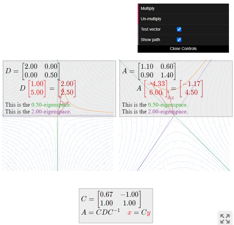
Describe how the matrix

\[ A = \frac 1{5}\left(\begin{array}{cc}13&-2\\-3&12\end{array}\right) \nonumber \]

acts on the plane.

Solution

First we diagonalize \(A\). The characteristic polynomial is

\[ f(\lambda) = \lambda^2 - \text{Tr}(A)\lambda + \det(A) = \lambda^2 - 5\lambda + 6 = (\lambda - 2)(\lambda - 3). \nonumber \]

Next we compute the \(2\)-eigenspace:

\[ (A-2I_3)v = 0 \iff \frac 15\left(\begin{array}{cc}3&-2\\-3&2\end{array}\right)v = 0 \;\xrightarrow{\text{RREF}}\; \left(\begin{array}{cc}1&-2/3\\0&0\end{array}\right)v = 0. \nonumber \]

The parametric form of this equation is \(x = 2/3y\text{,}\) so one eigenvector is \(v_1 = {2/3\choose 1}\). For the \(3\)-eigenspace, we have:

\[ (A-3I_3)v = 0 \iff \frac 15\left(\begin{array}{cc}-2&-2\\-3&-3\end{array}\right)v = 0 \;\xrightarrow{\text{RREF}}\; \left(\begin{array}{cc}1&1\\0&0\end{array}\right)v = 0. \nonumber \]

The parametric form of this equation is \(x = -y\text{,}\) so an eigenvector is \(v_2 = {-1\choose 1}\). It follows that \(A = CDC^{-1}\text{,}\) where

\[ C = \left(\begin{array}{cc}2/3&-1\\1&1\end{array}\right) \qquad D = \left(\begin{array}{cc}2&0\\0&3\end{array}\right). \nonumber \]

The diagonal matrix \(D\) scales the \(x\)-coordinate by \(2\) and the \(y\)-coordinate by \(3\). Therefore, it moves vectors farther from both the \(x\)-axis and the \(y\)-axis, but faster in the \(y\)-direction than the \(x\)-direction.

The matrix \(A\) does the same thing, in the \(v_1,v_2\)-coordinate system: multiplying a vector by \(A\) scales the \(v_1\)-coordinate by \(2\) and the \(v_2\)-coordinate by \(3\). Therefore, \(A\) moves vectors farther from the \(2\)-eigenspace and the \(3\)-eigenspace, but faster in the \(v_2\)-direction than the \(v_1\)-direction.

Figure \(\PageIndex{9}\): Dynamics of the matrices \(A\) and \(D\). Click “multiply” to multiply the colored points by \(D\) on the left and \(A\) on the right.

Example \(\PageIndex{15}\): Eigenvalues \(|\lambda_1| \lt 1,\,|\lambda_2| \lt 1\)

Describe how the matrix

\[ A' = \frac 1{30}\left(\begin{array}{cc}12&2\\3&13\end{array}\right) \nonumber \]

acts on the plane.

Solution

This is the inverse of the matrix \(A\) from the previous Example \(\PageIndex{14}\). In that example, we found \(A = CDC^{-1}\) for

\[ C = \left(\begin{array}{cc}2/3&-1\\1&1\end{array}\right) \qquad D = \left(\begin{array}{cc}2&0\\0&3\end{array}\right). \nonumber \]

Therefore, remembering that taking inverses reverses the order of multiplication, Fact 3.5.1 in Section 3.5, we have

\[ A' = A^{-1} = (CDC^{-1})^{-1} = (C^{-1})^{-1} D^{-1} C^{-1} = C\left(\begin{array}{cc}1/2&0\\0&1/3\end{array}\right)C^{-1}. \nonumber \]

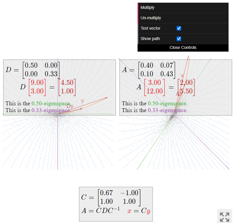
The diagonal matrix \(D^{-1}\) does the opposite of what \(D\) does: it scales the \(x\)-coordinate by \(1/2\) and the \(y\)-coordinate by \(1/3\). Therefore, it moves vectors closer to both coordinate axes, but faster in the \(y\)-direction. The matrix \(A'\) does the same thing, but with respect to the \(v_1,v_2\)-coordinate system.

Figure \(\PageIndex{10}\): Dynamics of the matrices \(A'\) and \(D^{-1}\). Click “multiply” to multiply the colored points by \(D^{-1}\) on the left and \(A'\) on the right.

Example \(\PageIndex{16}\): Eigenvalues \(|\lambda_1| = 1,\,|\lambda_2|\lt1\)

Describe how the matrix

\[ A = \frac 16\left(\begin{array}{cc}5&-1\\-2&4\end{array}\right) \nonumber \]

acts on the plane.

Solution

First we diagonalize \(A\). The characteristic polynomial is

\[ f(\lambda) = \lambda^2 - \text{Tr}(A)\lambda + \det(A) = \lambda^2 - \frac 32\lambda + \frac 12 = (\lambda - 1)\left(\lambda - \frac 12\right). \nonumber \]

Next we compute the \(1\)-eigenspace:

\[ (A-I_3)v = 0 \iff \frac 16\left(\begin{array}{cc}-1&-1\\-2&-2\end{array}\right)v = 0 \;\xrightarrow{\text{RREF}}\; \left(\begin{array}{cc}1&1\\0&0\end{array}\right)v = 0. \nonumber \]

The parametric form of this equation is \(x = -y\text{,}\) so one eigenvector is \(v_1 = {-1\choose 1}\). For the \(1/2\)-eigenspace, we have:

\[ \left(A-\frac 12I_3\right)v = 0 \iff \frac 16\left(\begin{array}{cc}2&-1\\-2&1\end{array}\right)v = 0 \;\xrightarrow{\text{RREF}}\; \left(\begin{array}{cc}1&-1/2 \\ 0&0\end{array}\right)v = 0. \nonumber \]

The parametric form of this equation is \(x = 1/2y\text{,}\) so an eigenvector is \(v_2 = {1/2\choose 1}\). It follows that \(A = CDC^{-1}\text{,}\) where

\[ C = \left(\begin{array}{cc}-1&1/2 \\ 1&1\end{array}\right) \qquad D = \left(\begin{array}{cc}1&0\\0&1/2\end{array}\right). \nonumber \]

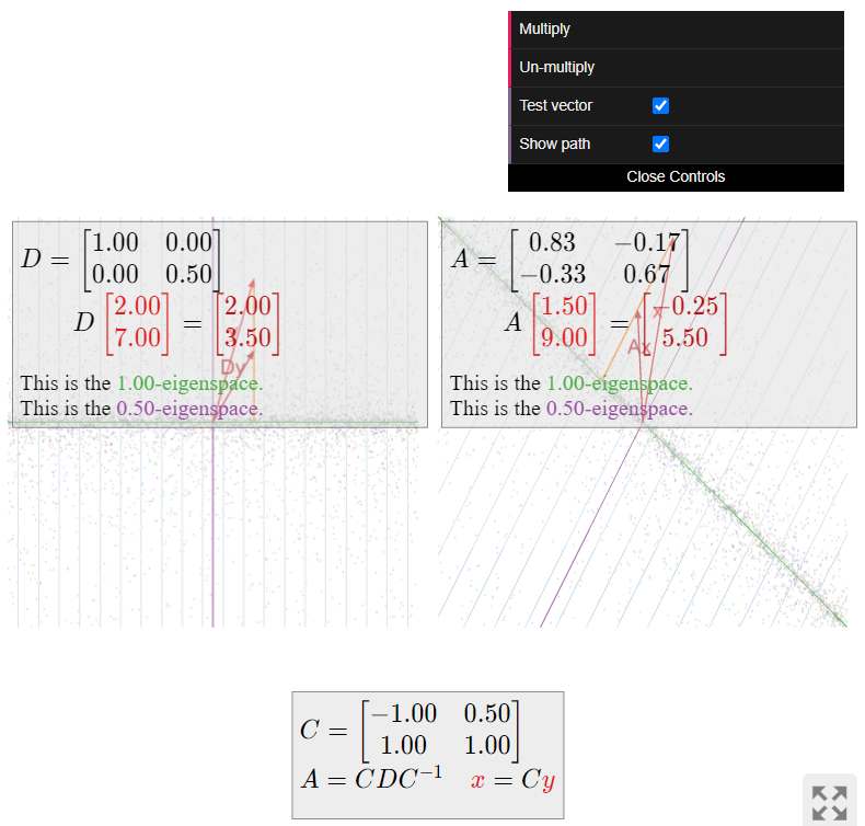
The diagonal matrix \(D\) scales the \(y\)-coordinate by \(1/2\) and does not move the \(x\)-coordinate. Therefore, it simply moves vectors closer to the \(x\)-axis along vertical lines. The matrix \(A\) does the same thing, in the \(v_1,v_2\)-coordinate system: multiplying a vector by \(A\) scales the \(v_2\)-coordinate by \(1/2\) and does not change the \(v_1\)-coordinate. Therefore, \(A\) “sucks vectors into the \(1\)-eigenspace” along lines parallel to \(v_2\).

Figure \(\PageIndex{11}\): Dynamics of the matrices \(A\) and \(D\). Click “multiply” to multiply the colored points by \(D\) on the left and \(A\) on the right.

Example \(\PageIndex{17}\): Interactive: A diagonalizable \(3\times 3\) matrix

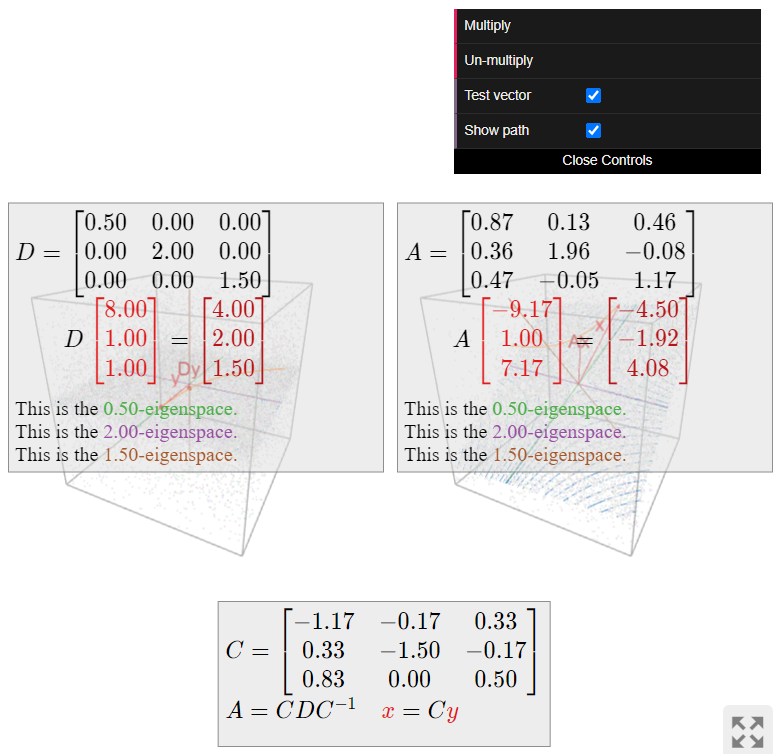
The diagonal matrix

\[ D = \left(\begin{array}{ccc}1/2&0&0\\0&2&0\\0&0&3/2\end{array}\right) \nonumber \]

scales the \(x\)-coordinate by \(1/2\text{,}\) the \(y\)-coordinate by \(2\text{,}\) and the \(z\)-coordinate by \(3/2\). Looking straight down at the \(xy\)-plane, the points follow parabolic paths taking them away from the \(x\)-axis and toward the \(y\)-axis. The \(z\)-coordinate is scaled by \(3/2\text{,}\) so points fly away from the \(xy\)-plane in that direction.

If \(A = CDC^{-1}\) for some invertible matrix \(C\text{,}\) then \(A\) does the same thing as \(D\text{,}\) but with respect to the coordinate system defined by the columns of \(C\).

Figure \(\PageIndex{12}\): Dynamics of the matrices \(A\) and \(D\). Click “multiply” to multiply the colored points by \(D\) on the left and \(A\) on the right.

Algebraic and Geometric Multiplicity

In this subsection, we give a variant of Theorem \(\PageIndex{1}\) that provides another criterion for diagonalizability. It is stated in the language of multiplicities of eigenvalues.

In algebra, we define the multiplicity of a root \(\lambda_0\) of a polynomial \(f(\lambda)\) to be the number of factors of \(\lambda-\lambda_0\) that divide \(f(\lambda).\) For instance, in the polynomial

\[ f(\lambda) = -\lambda^3 + 4\lambda^2 - 5\lambda + 2 = -(\lambda-1)^2(\lambda-2), \nonumber \]

the root \(\lambda_0=2\) has multiplicity \(1\text{,}\) and the root \(\lambda_0=1\) has multiplicity \(2\).

Definition \(\PageIndex{2}\): Algebraic Multiplicity and Geometric Multiplicity

Let \(A\) be an \(n\times n\) matrix, and let \(\lambda\) be an eigenvalue of \(A\).

1. The algebraic multiplicity of \(\lambda\) is its multiplicity as a root of the characteristic polynomial of \(A\).
2. The geometric multiplicity of \(\lambda\) is the dimension of the \(\lambda\)-eigenspace.

Since the \(\lambda\)-eigenspace of \(A\) is \(\text{Nul}(A-\lambda I_n)\text{,}\) its dimension is the number of free variables in the system of equations \((A - \lambda I_n)x=0\text{,}\) i.e., the number of columns without pivots in the matrix \(A-\lambda I_n\).

Example \(\PageIndex{18}\)

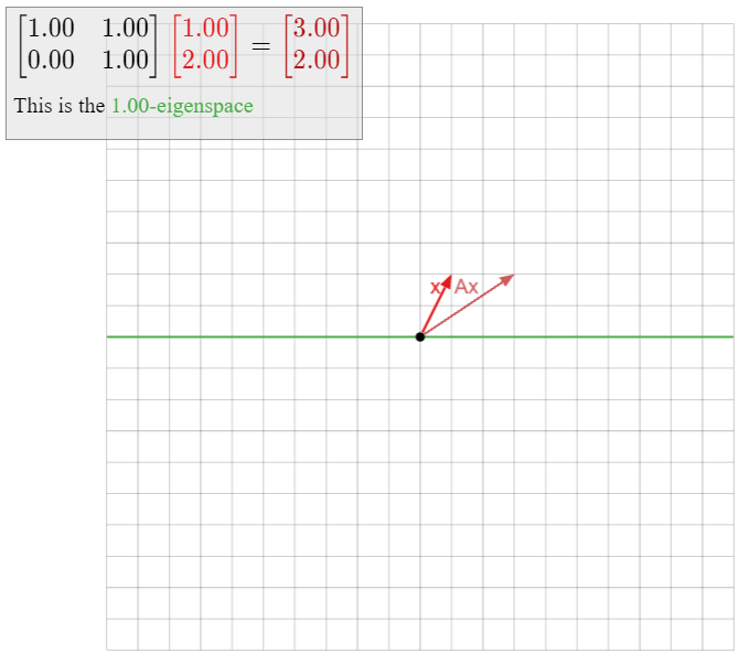
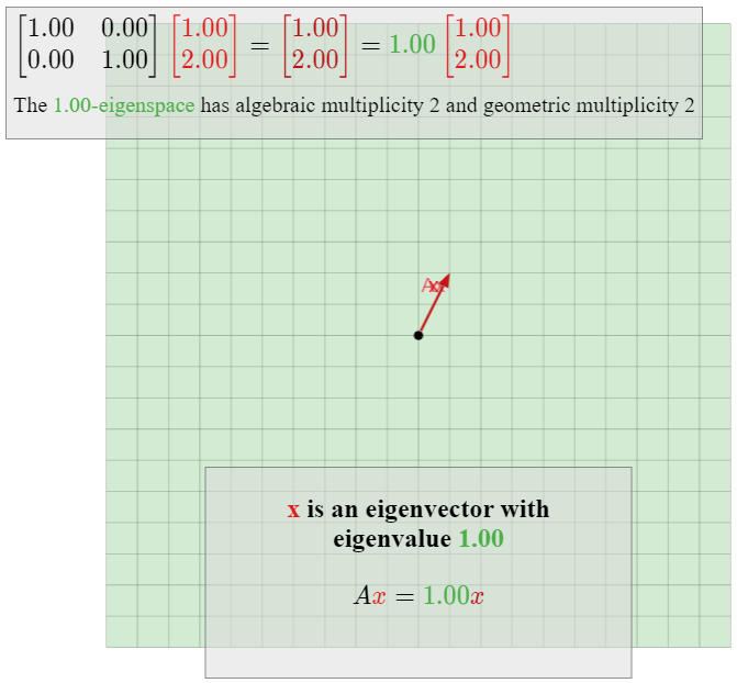
The shear matrix

\[ A = \left(\begin{array}{cc}1&1\\0&1\end{array}\right) \nonumber \]

has only one eigenvalue \(\lambda=1\). The characteristic polynomial of \(A\) is \(f(\lambda) = (\lambda-1)^2\text{,}\) so \(1\) has algebraic multiplicity \(2\text{,}\) as it is a double root of \(f\). On the other hand, we showed in Example \(\PageIndex{9}\) that the \(1\)-eigenspace of \(A\) is the \(x\)-axis, so the geometric multiplicity of \(1\) is equal to \(1\). This matrix is not diagonalizable.

Figure \(\PageIndex{13}\): Eigenspace of the shear matrix, with multiplicities.

The identity matrix

\[ I_2 = \left(\begin{array}{cc}1&0\\0&1\end{array}\right) \nonumber \]

also has characteristic polynomial \((\lambda-1)^2\text{,}\) so the eigenvalue \(1\) has algebraic multiplicity \(2\). Since every nonzero vector in \(\mathbb{R}^2 \) is an eigenvector of \(I_2\) with eigenvalue \(1\text{,}\) the \(1\)-eigenspace is all of \(\mathbb{R}^2 \text{,}\) so the geometric multiplicity is \(2\) as well. This matrix is diagonal.

Figure \(\PageIndex{14}\): Eigenspace of the identity matrix, with multiplicities.

Example \(\PageIndex{19}\)

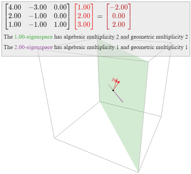
Continuing with Example \(\PageIndex{8}\), let

\[ A = \left(\begin{array}{ccc}4&-2&0\\2&-1&0\\1&-1&1\end{array}\right). \nonumber \]

The characteristic polynomial is \(f(\lambda) = -(\lambda-1)^2(\lambda-2)\text{,}\) so that \(1\) and \(2\) are the eigenvalues, with algebraic multiplicities \(2\) and \(1\text{,}\) respectively. We computed that the \(1\)-eigenspace is a plane and the \(2\)-eigenspace is a line, so that \(1\) and \(2\) also have geometric multiplicities \(2\) and \(1\text{,}\) respectively. This matrix is diagonalizable.

Figure \(\PageIndex{15}\): The green plane is the \(1\)-eigenspace of \(A\text{,}\) and the violet line is the \(2\)-eigenspace. Hence the geometric multiplicity of the \(1\)-eigenspace is \(2\text{,}\) and the geometric multiplicity of the \(2\)-eigenspace is \(1\).

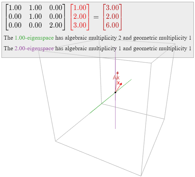
In Example \(\PageIndex{11}\), we saw that the matrix

\[ A = \left(\begin{array}{ccc}1&1&0\\0&1&0\\0&0&2\end{array}\right) \nonumber \]

also has characteristic polynomial \(f(\lambda) = -(\lambda-1)^2(\lambda-2)\text{,}\) so that \(1\) and \(2\) are the eigenvalues, with algebraic multiplicities \(2\) and \(1\text{,}\) respectively. In this case, however, both eigenspaces are lines, so that both eigenvalues have geometric multiplicity \(1\). This matrix is not diagonalizable.

Figure \(\PageIndex{16}\): Both eigenspaces of \(A\) are lines, so they both have geometric multiplicity \(1\).

We saw in the above examples that the algebraic and geometric multiplicities need not coincide. However, they do satisfy the following fundamental inequality, the proof of which is beyond the scope of this text.

Theorem \(\PageIndex{2}\): Algebraic and Geometric Multiplicity

Let \(A\) be a square matrix and let \(\lambda\) be an eigenvalue of \(A\). Then

\[ 1 \leq \text{(the geometric multiplicity of $\lambda$)} \leq \text{(the algebraic multiplicity of $\lambda$)}. \nonumber \]

In particular, if the algebraic multiplicity of \(\lambda\) is equal to \(1\text{,}\) then so is the geometric multiplicity.

Note \(\PageIndex{4}\)

If \(A\) has an eigenvalue \(\lambda\) with algebraic multiplicity \(1\text{,}\) then the \(\lambda\)-eigenspace is a line.

We can use Theorem \(\PageIndex{2}\) to give another criterion for diagonalizability (in addition to Theorem \(\PageIndex{1}\)).

Theorem \(\PageIndex{3}\): Diagonalization Theorem, Variant

Let \(A\) be an \(n\times n\) matrix. The following are equivalent:

1. \(A\) is diagonalizable.
2. The sum of the geometric multiplicities of the eigenvalues of \(A\) is equal to \(n\).
3. The sum of the algebraic multiplicities of the eigenvalues of \(A\) is equal to \(n\text{,}\) and for each eigenvalue, the geometric multiplicity equals the algebraic multiplicity.

Proof

We will show \(1\implies 2\implies 3\implies 1\). First suppose that \(A\) is diagonalizable. Then \(A\) has \(n\) linearly independent eigenvectors \(v_1,v_2,\ldots,v_n\). This implies that the sum of the geometric multiplicities is at least \(n\text{:}\) for instance, if \(v_1,v_2,v_3\) have the same eigenvalue \(\lambda\text{,}\) then the geometric multiplicity of \(\lambda\) is at least \(3\) (as the \(\lambda\)-eigenspace contains three linearly independent vectors), and so on. But the sum of the algebraic multiplicities is greater than or equal to the sum of the geometric multiplicities by Theorem \(\PageIndex{2}\), and the sum of the algebraic multiplicities is at most \(n\) because the characteristic polynomial has degree \(n\). Therefore, the sum of the geometric multiplicities equals \(n\).

Now suppose that the sum of the geometric multiplicities equals \(n\). As above, this forces the sum of the algebraic multiplicities to equal \(n\) as well. As the algebraic multiplicities are all greater than or equal to the geometric multiplicities in any case, this implies that they are in fact equal.

Finally, suppose that the third condition is satisfied. Then the sum of the geometric multiplicities equals \(n\). Suppose that the distinct eigenvectors are \(\lambda_1,\lambda_2,\ldots,\lambda_k\text{,}\) and that \(\mathcal{B}_i\) is a basis for the \(\lambda_i\)-eigenspace, which we call \(V_i\). We claim that the collection \(\mathcal{B} = \{v_1,v_2,\ldots,v_n\}\) of all vectors in all of the eigenspace bases \(\mathcal{B}_i\) is linearly independent. Consider the vector equation

\[ 0 = c_1v_1 + c_2v_2 + \cdots + c_nv_n. \nonumber \]

Grouping the eigenvectors with the same eigenvalues, this sum has the form

\[ 0 = \text{(something in $V_1$)} + \text{(something in $V_2$)} + \cdots + \text{(something in $V_k$)}. \nonumber \]

Since eigenvectors with distinct eigenvalues are linearly independent, Fact 5.1.1 in Section 5.1, each “something in \(V_i\)” is equal to zero. But this implies that all coefficients \(c_1,c_2,\ldots,c_n\) are equal to zero, since the vectors in each \(\mathcal{B}_i\) are linearly independent. Therefore, \(A\) has \(n\) linearly independent eigenvectors, so it is diagonalizable.

The first part of the third statement simply says that the characteristic polynomial of \(A\) factors completely into linear polynomials over the real numbers: in other words, there are no complex (non-real) roots. The second part of the third statement says in particular that for any diagonalizable matrix, the algebraic and geometric multiplicities coincide.

Note \(\PageIndex{5}\)

Let \(A\) be a square matrix and let \(\lambda\) be an eigenvalue of \(A\). If the algebraic multiplicity of \(\lambda\) does not equal the geometric multiplicity, then \(A\) is not diagonalizable.

The examples at the beginning of this subsection illustrate the theorem. Here we give some general consequences for diagonalizability of \(2\times 2\) and \(3\times 3\) matrices.

Example \(\PageIndex{20}\): Diagonalizability of \(2\times 2\) Matrices

Let \(A\) be a \(2\times 2\) matrix. There are four cases:

1. \(A\) has two different eigenvalues. In this case, each eigenvalue has algebraic and geometric multiplicity equal to one. This implies \(A\) is diagonalizable. For example: \[A=\left(\begin{array}{cc}1&7\\0&2\end{array}\right).\nonumber\]
2. \(A\) has one eigenvalue \(\lambda\) of algebraic and geometric multiplicity \(2\). To say that the geometric multiplicity is \(2\) means that \(\text{Nul}(A-\lambda I_2) = \mathbb{R}^2 \text{,}\) i.e., that every vector in \(\mathbb{R}^2 \) is in the null space of \(A-\lambda I_2\). This implies that \(A-\lambda I_2\) is the zero matrix, so that \(A\) is the diagonal matrix \(\lambda I_2\). In particular, \(A\) is diagonalizable. For example: \[A=\left(\begin{array}{cc}1&0\\0&1\end{array}\right).\nonumber\]
3. \(A\) has one eigenvalue \(\lambda\) of algebraic multiplicity \(2\) and geometric multiplicity \(1\). In this case, \(A\) is not diagonalizable, by part 3 of Theorem \(\PageIndex{3}\). For example, a shear: \[A=\left(\begin{array}{cc}1&1\\0&1\end{array}\right).\nonumber\]
4. \(A\) has no eigenvalues. This happens when the characteristic polynomial has no real roots. In particular, \(A\) is not diagonalizable. For example, a rotation: \[A=\left(\begin{array}{cc}1&-1\\1&1\end{array}\right).\nonumber\]

Example \(\PageIndex{21}\): Diagonalizability of \(3\times 3\) Matrices

Let \(A\) be a \(3\times 3\) matrix. We can analyze the diagonalizability of \(A\) on a case-by-case basis, as in the previous Example \(\PageIndex{20}\).

1. \(A\) has three different eigenvalues. In this case, each eigenvalue has algebraic and geometric multiplicity equal to one. This implies \(A\) is diagonalizable. For example: \[A=\left(\begin{array}{ccc}1&7&4\\0&2&3\\0&0&-1\end{array}\right).\nonumber\]
2. \(A\) has two distinct eigenvalues \(\lambda_1,\lambda_2\). In this case, one has algebraic multiplicity one and the other has algebraic multiplicity two; after reordering, we can assume \(\lambda_1\) has multiplicity \(1\) and \(\lambda_2\) has multiplicity \(2\). This implies that \(\lambda_1\) has geometric multiplicity \(1\text{,}\) so \(A\) is diagonalizable if and only if the \(\lambda_2\)-eigenspace is a plane. For example: \[A=\left(\begin{array}{ccc}1&7&4\\0&2&0\\0&0&2\end{array}\right).\nonumber\] On the other hand, if the geometric multiplicity of \(\lambda_2\) is \(1\text{,}\) then \(A\) is not diagonalizable. For example: \[A=\left(\begin{array}{ccc}1&7&4\\0&2&1\\0&0&2\end{array}\right).\nonumber\]
3. \(A\) has only one eigenvalue \(\lambda\). If the algebraic multiplicity of \(\lambda\) is \(1\text{,}\) then \(A\) is not diagonalizable. This happens when the characteristic polynomial has two complex (non-real) roots. For example: \[A=\left(\begin{array}{ccc}1&-1&0\\1&1&0\\0&0&2\end{array}\right).\nonumber\] Otherwise, the algebraic multiplicity of \(\lambda\) is equal to \(3\). In this case, if the geometric multiplicity is \(1\text{:}\) \[A=\left(\begin{array}{ccc}1&1&1\\0&1&1\\0&0&1\end{array}\right)\nonumber\] or \(2\text{:}\) \[A=\left(\begin{array}{ccc}1&0&1\\0&1&1\\0&0&1\end{array}\right)\nonumber\] then \(A\) is not diagonalizable. If the geometric multiplicity is \(3\text{,}\) then \(\text{Nul}(A-\lambda I_3) = \mathbb{R}^3 \text{,}\) so that \(A-\lambda I_3\) is the zero matrix, and hence \(A = \lambda I_3\). Therefore, in this case \(A\) is necessarily diagonal, as in: \[A=\left(\begin{array}{ccc}1&0&0\\0&1&0\\0&0&1\end{array}\right).\nonumber\]

Similarity and Multiplicity

Recall from Fact 5.3.2 in Section 5.3 that similar matrices have the same eigenvalues. It turns out that both notions of multiplicity of an eigenvalue are preserved under similarity.

Theorem \(\PageIndex{4}\)

Let \(A\) and \(B\) be similar \(n\times n\) matrices, and let \(\lambda\) be an eigenvalue of \(A\) and \(B\). Then:

1. The algebraic multiplicity of \(\lambda\) is the same for \(A\) and \(B\).
2. The geometric multiplicity of \(\lambda\) is the same for \(A\) and \(B\).

Proof

Since \(A\) and \(B\) have the same characteristic polynomial, the multiplicity of \(\lambda\) as a root of the characteristic polynomial is the same for both matrices, which proves the first statement. For the second, suppose that \(A = CBC^{-1}\) for an invertible matrix \(C\). By Fact 5.3.3 in Section 5.3, the matrix \(C\) takes eigenvectors of \(B\) to eigenvectors of \(A\text{,}\) both with eigenvalue \(\lambda\).

Let \(\{v_1,v_2,\ldots,v_k\}\) be a basis of the \(\lambda\)-eigenspace of \(B\). We claim that \(\{Cv_1,Cv_2,\ldots,Cv_k\}\) is linearly independent. Suppose that

\[ c_1Cv_1 + c_2Cv_2 + \cdots + c_kCv_k = 0. \nonumber \]

Regrouping, this means

\[ C\bigl(c_1v_1 + c_2v_2 + \cdots + c_kv_k\bigr) = 0. \nonumber \]

By Theorem 5.1.1 in Section 5.1, the null space of \(C\) is trivial, so this implies

\[ c_1v_1 + c_2v_2 + \cdots + c_kv_k = 0. \nonumber \]

Since \(v_1,v_2,\ldots,v_k\) are linearly independent, we get \(c_1=c_2=\cdots=c_k=0\text{,}\) as desired.

By the previous paragraph, the dimension of the \(\lambda\)-eigenspace of \(A\) is greater than or equal to the dimension of the \(\lambda\)-eigenspace of \(B\). By symmetry (\(B\) is similar to \(A\) as well), the dimensions are equal, so the geometric multiplicities coincide.

For instance, the four matrices in Example \(\PageIndex{20}\) are not similar to each other, because the algebraic and/or geometric multiplicities of the eigenvalues do not match up. Or, combined with the above Theorem \(\PageIndex{3}\), we see that a diagonalizable matrix cannot be similar to a non-diagonalizable one, because the algebraic and geometric multiplicities of such matrices cannot both coincide.

Example \(\PageIndex{22}\)

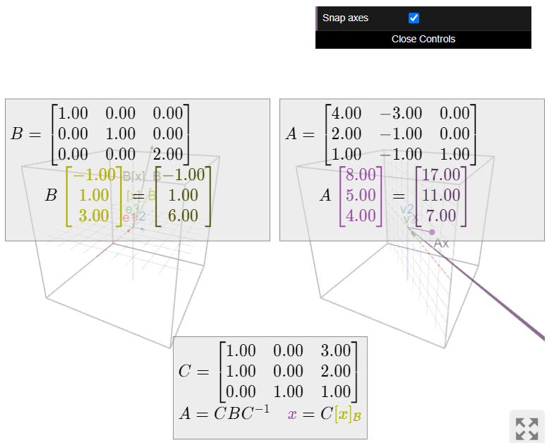
Continuing with this Example \(\PageIndex{8}\), let

\[ A = \left(\begin{array}{ccc}4&-3&0\\2&-1&0\\1&-1&1\end{array}\right). \nonumber \]

This is a diagonalizable matrix that is similar to

\[ D = \left(\begin{array}{ccc}1&0&0\\0&1&0\\0&0&2\end{array}\right)\quad\text{using the matrix}\quad C = \left(\begin{array}{ccc}1&0&3\\1&0&2\\0&1&1\end{array}\right). \nonumber \]

The \(1\)-eigenspace of \(D\) is the \(xy\)-plane, and the \(2\)-eigenspace is the \(z\)-axis. The matrix \(C\) takes the \(xy\)-plane to the \(1\)-eigenspace of \(A\text{,}\) which is again a plane, and the \(z\)-axis to the \(2\)-eigenspace of \(A\text{,}\) which is again a line. This shows that the geometric multiplicities of \(A\) and \(D\) coincide.

Figure \(\PageIndex{17}\): The matrix \(C\) takes the \(xy\)-plane to the \(1\)-eigenspace of \(A\) (the grid) and the \(z\)-axis to the \(2\)-eigenspace (the green line).

The converse of Theorem \(\PageIndex{4}\) is false: there exist matrices whose eigenvectors have the same algebraic and geometric multiplicities, but which are not similar. See Example \(\PageIndex{23}\) below. However, for \(2\times 2\) and \(3\times 3\) matrices whose characteristic polynomial has no complex (non-real) roots, the converse of Theorem \(\PageIndex{4}\) is true. (We will handle the case of complex roots in Section 5.5.)

Example \(\PageIndex{23}\): Matrices that look similar but are not

Show that the matrices

\[A=\left(\begin{array}{cccc}0&0&0&0\\0&0&1&0\\0&0&0&1\\0&0&0&0\end{array}\right)\quad\text{and}\quad B=\left(\begin{array}{cccc}0&1&0&0\\0&0&0&0\\0&0&0&1\\0&0&0&0\end{array}\right)\nonumber\]

have the same eigenvalues with the same algebraic and geometric multiplicities, but are not similar.

Solution

These matrices are upper-triangular. They both have characteristic polynomial \(f(\lambda) = \lambda^4\text{,}\) so they both have one eigenvalue \(0\) with algebraic multiplicity \(4\). The \(0\)-eigenspace is the null space, Fact 5.1.2 in Section 5.1, which has dimension \(2\) in each case because \(A\) and \(B\) have two columns without pivots. Hence \(0\) has geometric multiplicity \(2\) in each case.

To show that \(A\) and \(B\) are not similar, we note that

\[A^2=\left(\begin{array}{cccc}0&0&0&0\\0&0&0&1\\0&0&0&0\\0&0&0&0\end{array}\right)\quad\text{and}\quad B^2=\left(\begin{array}{cccc}0&0&0&0\\0&0&0&0\\0&0&0&0\\0&0&0&0\end{array}\right),\nonumber\]

as the reader can verify. If \(A = CBC^{-1}\) then by Recipe: Compute Powers of a Diagonalizable Matrix, we have

\[ A^2 = CB^2C^{-1} = C0C^{-1} = 0, \nonumber \]

which is not the case.

On the other hand, suppose that \(A\) and \(B\) are diagonalizable matrices with the same characteristic polynomial. Since the geometric multiplicities of the eigenvalues coincide with the algebraic multiplicities, which are the same for \(A\) and \(B\text{,}\) we conclude that there exist \(n\) linearly independent eigenvectors of each matrix, all of which have the same eigenvalues. This shows that \(A\) and \(B\) are both similar to the same diagonal matrix. Using the transitivity property, Proposition 5.3.1 in Section 5.3, of similar matrices, this shows:

Note \(\PageIndex{6}\)

Diagonalizable matrices are similar if and only if they have the same characteristic polynomial, or equivalently, the same eigenvalues with the same algebraic multiplicities.

Example \(\PageIndex{24}\)

Show that the matrices

\[A=\left(\begin{array}{ccc}1&7&2\\0&-1&3\\0&0&4\end{array}\right)\quad\text{and}\quad B=\left(\begin{array}{ccc}1&0&0\\-2&4&0\\-5&-4&-1\end{array}\right)\nonumber\]

are similar.

Solution

Both matrices have the three distinct eigenvalues \(1,-1,4\). Hence they are both diagonalizable, and are similar to the diagonal matrix

\[ \left(\begin{array}{ccc}1&0&0\\0&-1&0\\0&0&4\end{array}\right). \nonumber \]

By the transitivity property, Proposition 5.3.1 in Section 5.3, of similar matrices, this implies that \(A\) and \(B\) are similar to each other.

Example \(\PageIndex{25}\): Diagonal matrices with the same entries are similar

Any two diagonal matrices with the same diagonal entries (possibly in a different order) are similar to each other. Indeed, such matrices have the same characteristic polynomial. We saw this phenomenon in Example \(\PageIndex{5}\), where we noted that

\[\left(\begin{array}{ccc}1&0&0\\0&2&0\\0&0&3\end{array}\right)=\left(\begin{array}{ccc}0&0&1\\0&1&0\\1&0&0\end{array}\right)\left(\begin{array}{ccc}3&0&0\\0&2&0\\0&0&1\end{array}\right)\left(\begin{array}{ccc}0&0&1\\0&1&0\\1&0&0\end{array}\right)^{-1}.\nonumber\]